Structural connectivity dMRI

This tutorial was created by Joan Amos.

Email: joan@std.uestc.edu.cn Github: @Joanone

References:

The steps used for this tutorial were from:

• https://github.com/civier/HCP-dMRI-connectome
• https://andysbrainbook.readthedocs.io/en/latest/MRtrix/MRtrix_Course/MRtrix_00_Diffusion_Overview.html
• https://mrtrix.readthedocs.io/en/latest/quantitative_structural_connectivity/structural_connectome.html

Data Description

Reference:

The single subject data (T1w structural and diffusion) used in this tutorial has been minimally preprocessed and was downloaded from the open available source:

db.humanconnectome.org

Download demo data:

Demo data can also be downloaded using these links below.

• https://drive.google.com/file/d/1bj-Tz2xLGn0L05CveOYnzTgkewc_IU5F/view?usp=drive_link [T1w structural data]
• https://drive.google.com/file/d/193ZaUmXbT59IoXoAJ-Y1pf_wgdSHdKpR/view?usp=drive_link [Diffusion data]

Assumptions:

• You have neurodesk already running from your chrome browser.
• You have sufficient disk space to successfully implement the structural connectivity.
• The structural and diffusion sample data have been unzipped in the mounted storage directory.

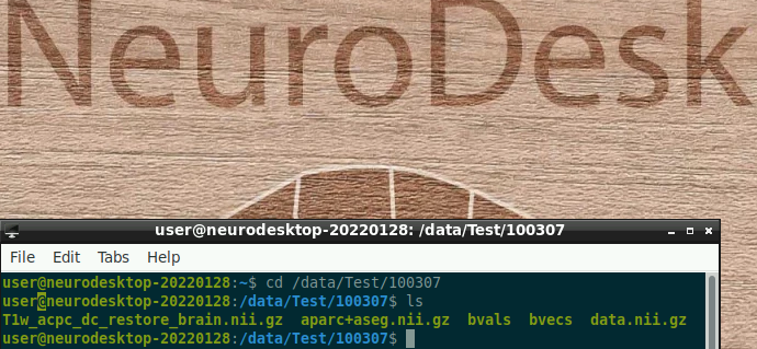
Sample Subject (100307) directory tree structure should include these input files:

• aparc+aseg.nii.gz
• T1w_acpc_dc_restore_brain.nii.gz
• bvals
• bvecs
• data.nii.gz

Navigate to the mounted storage → more data → Create a new folder of your choice → copy the required input files into a folder → 100307

N/B: The subfolder used in this tutorial was tagged “Test”

Open a terminal in neurodesk and confirm your input files:

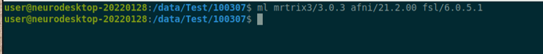
Activate mrtrix3, fsl and afni software versions of your choice in the neurodesk terminal

N/B: mrtrix3 (3.0.3), afni (21.2.00), fsl(6.0.5.1) versions were used in this tutorial. For reproducibility, the same versions can be maintained.

Step 1: Further pre-processing

Extract data.nii.gz to enable memory-mapping. The extracted files are about 4.5GB:

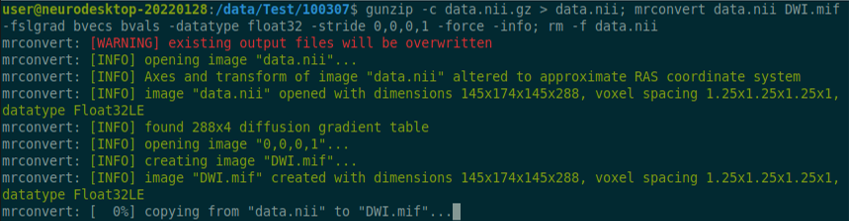
Perform mrconvert:

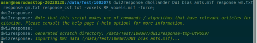
Extract the response function. Uses stride 0,0,0,1:

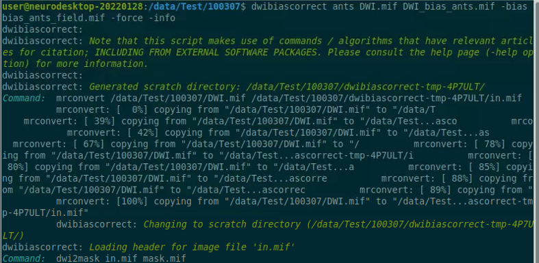
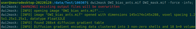
Generate mask:

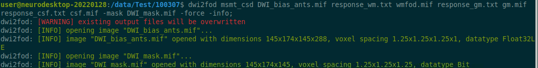
Generate Fibre Orientation Distributions (FODs):

Perform normalization:

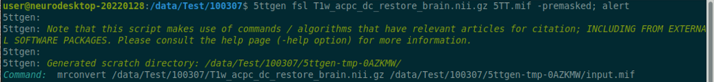
Generate a 5 tissue image:

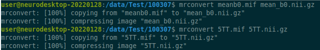
Convert the B0 and 5TT image to a compressed format:

Use “fslroi” to extract the first volume of the segmented dataset which corresponds to the Grey Matter Segmentation:

Use “flirt” command to perform coregisteration:

Convert the transformation matrix to a format readable by MRtrix3:

Coregister the anatomical image to the diffusion image:

Create the seed boundary which separates the grey from the white matter. The command “5tt2gmwmi” denotes (5 tissue type(segmentation) to grey matter/white matter interface):

Step 2: Tractogram construction

The probabilistic tractography which is the default in MRtrix is used in this tutorial. The default method is the iFOD2 algorithm. The number of streamlines used is 10 million, this was chosen to save computational time:

Proceed to Step 3 when the process above is completed (100%).

Step 3: SIFT2 construction

The generated streamlines can be refined with tcksift2 to counterbalance the overfitting. This creates a text file containing weights for each voxel in the brain:

Step 4: Connectome construction

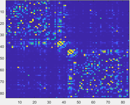
In constructing the connectome, the desikan-killany atlas which includes the cortical and sub-cortical regions (84 regions) was used.

Copy the “FreeSurferColorLUT.txt” file from the ml freesurfer 7.2.0 singularity container to the subject’s folder:

Copy the “fs_default.txt” file from the ml mrtrix3 3.0.3 singularity container to the subject’s folder:

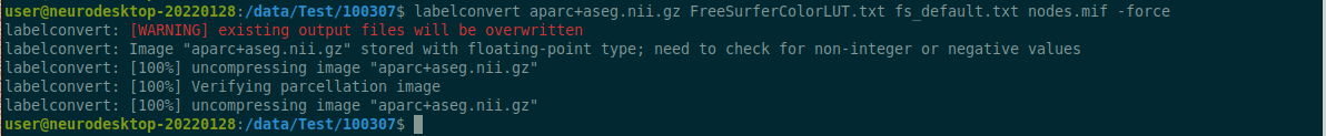
The command labelconvert uses the parcellation and segmentation output of FreeSurfer to create a new parcellated file in .mif format:

Perform nodes co-registeration:

Create a whole-brain connectome which denotes the streamlines between each parcellation pair in the atlas. The “symmetric” option makes the lower and upper diagonal the same, the “scale_invnodevol” option scales the connectome by the inverse of the size of the node:

Viewing the connectome

The generated nodes.csv file can be viewed outside neurodesk as a matrix in Matlab.

connectome=importdata('nodes.csv');
imagesc(connectome,[0 1])

Congratulations on constructing a single subject’s structural connectome with neurodesk! Running multiple subjects would require scripting. Kindly consult the references above.