Functional Imaging

• 1: Connectome Workbench
• 2: Using fmriprep with neurodesk on an HPC
• 3: Using mriqc with neurodesk on HPC
• 4: PhysIO
• 5: A batch scripting example for PhysIO toolbox
• 6: Statistical Parametric Mapping (SPM)

1 - Connectome Workbench

This tutorial was created by Fernanda L. Ribeiro.

Email: fernanda.ribeiro@uq.edu.au

Github: @felenitaribeiro

Twitter: @NandaRibeiro93

This tutorial documents how to use Connectome Workbench on NeuroDesk for visualizing the 7T HCP Retinotopy Dataset.

Download data

1. First, make sure you register for the Human Connectome Project Open Access Data: https://www.humanconnectome.org/study/hcp-young-adult/data-use-terms

2. Register to the BALSA database: https://balsa.wustl.edu/.

3. Login and download the scene files containing the retinotopic maps available at: https://balsa.wustl.edu/study/9Zkk.

These files include preprocessed collated data from 181 participants, including retinotopic, curvature, midthickness, and myelin maps.

4. Finally, unzip the S1200_7T_Retinotopy_9Zkk.zip file.

Visualizing scene files

Using Connectome Workbench, you can load “.scene” files and visualize all individuals’ retinotopic maps. To do so, follow the next steps:

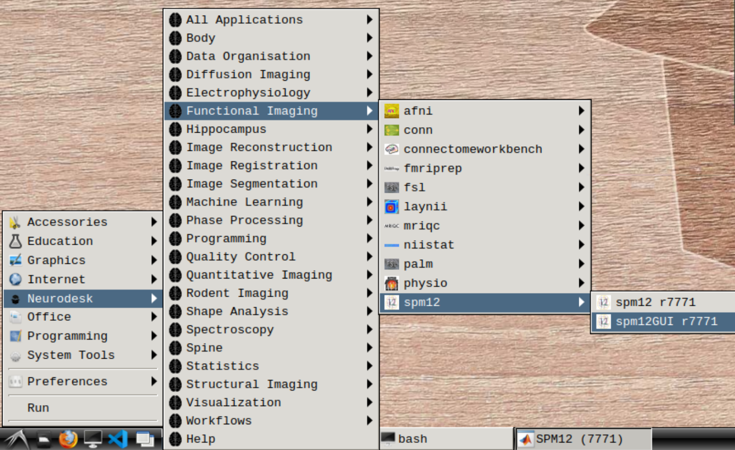
1. In the application menu, navigate to Neurodesk → functional imaging → connectomeworkbench → connectomeworkbench 1.5.0

2. On the terminal shell that pops up, type in:

wb_view

3. Click on “Open Other”

and search for a scene file

in the path where your data is

Finally, select the desired file and open it:

4. On the ‘Scenes’ window that will pop up, select the first option.

The default images are the average maps.

5. To change the displayed images for an individual’s data instead, click on the first ticked dropdown menu

and select “S1200_7T_Retinotopy181.All.Fit1_PolarAngle_MSMALL.32k_fs_LR.dscalar.nii”:

6. Now, you should be able to select specific maps from the dropdown menu on the right. For example, here we have the first individual polar angle map (top left):

Now we have the fifth:

7. You can do the same for the other functional maps by navigating through the tabs at the top.

2 - Using fmriprep with neurodesk on an HPC

This tutorial was created by Kelly G. Garner.

Github: @kel_github

This workflow documents how to use fmriprep with neurodesk and provides some details that may help you troubleshoot some common problems I found along the way.

An example notebook can be found here: https://github.com/NeuroDesk/example-notebooks/blob/main/books/functional_imaging/fmriprep_example.ipynb

Assumptions

• Your data is already in BIDS format
• You plan to run fmriprep using Neurodesk
• You have a copy of the freesurfer license file (freesurfer.txt), that can be read from the file system using Neurodesk

Steps

Launch Neurodesk

From the launcher, click the Neurodesktop icon:

Open fmriprep

Now you’re in Neurodesk, use the menus to first open the neurodesk options

and then select fMRIPrep. Note that the latest version will be the lowest on the dropdown list:

This will open a terminal window where fMRIPrep is ready and waiting at your fingertips - woohoo!

Setting up fmriprep command

You can now enter your fmriprep command straight into the command line in the newly opened terminal. Here is a quick guide to the command I have used with the options I have found most useful. Note that fMRIPrep requests the path to the freesurfer license file, which should be somewhere in your system for neurodesk to read - e.g. in ’neurodesktop-storage'.

export ITK_GLOBAL_DEFAULT_NUMBER_OF_THREADS=6 # specify the number of threads you want to use

fmriprep /path/to/your/data \ # this is the top level of your data folder
         /path/to/your/data/derivatives \ # where you want fmriprep output to be saved
         participant \ # this tells fmriprep to analyse at the participant level
         --fs-license-file /path/to/your/freesurfer.txt \ # where the freesurfer license file is
         --output-spaces T1w MNI152NLin2009cAsym fsaverage fsnative \ 
         --participant-label 01 \ # put what ever participant labels you want to analyse
         --nprocs 6 --mem 10000 \ # fmriprep can be greedy on the hpc, make sure it is not
         --skip_bids_validation \ # its normally fine to skip this but do make sure your data are BIDS enough
         -v # be verbal fmriprep, tell me what you are doing

Then hit return and fMRIPrep should now be merrily working away on your data :)

Some common pitfalls I have learned from my mistakes (and sometimes from others)

1. If fmriprep hangs it could well be that you are out of disk space. Sometimes this is because fmriprep created a work directory in your home folder which is often limited on the HPC. Make sure fmriprep knows to use a work drectory in your scratch. you can specify this in the fmriprep command by using -w /path/to/the/work/directory/you/made

2. I learned the following from TomCat (@thomshaw92) - fMRIPrep can get confused between subjects when run in parallel. Parallelise with caution.

3. If running on a HPC, make sure to set the processor and memory limits, if not your job will get killed because it hogs all the resources.

3 - Using mriqc with neurodesk on HPC

This tutorial was created by Kelly G. Garner.

Github: @kel_github

This workflow documents how to use MRIQC with neurodesk and provides some details that may help you troubleshoot some common problems I found along the way.

Assumptions

• Your data is already in BIDS format
• You plan to run mriqc using Neurodesk

Steps

Launch Neurodesk

From the launcher, click the Neurodesktop icon:

Open MRIQC

Now you’re in Neurodesk, use the menus to first open the neurodesk options

and then select MRIQC. Note that the latest version will be the lowest on the dropdown list:

This will open a terminal window where MRIQC is ready and waiting at your fingertips - woohoo!

Setting up mriqc command

You can now enter the following mriqc commands straight into the command line in the newly opened terminal window.

export ITK_GLOBAL_DEFAULT_NUMBER_OF_THREADS=6 # specify the number of threads you want to use

mriqc /path/to/your/data \ # this is the top level of your data folder
         /path/to/your/data/derivatives \ # where you want mriqc output to be saved
         participant \ # this tells mriqc to analyse at the participant level
         --participant-label 01 \ # put what ever participant labels you want to analyse
         --work-dir /path/to/work/directory \ #useful to specify so your home directory definitely does not get clogged
         --nprocs 6 --mem_gb 10000 \ # mriqc can be greedy on the hpc, make sure it is not
         -v # be verbal mriqc, tell me what you are doing

Note that above I have set the processor and memory limits. This is because I was in this case running on an HPC, and I used those commands to stop MRIQC from hogging all the resources. You may want to skip those inputs if you’re running MRIQC locally.

OR: if you have run all the participants and you just want the group level report, use these mriqc commands instead:

mriqc /path/to/your/data \ # this is the top level of your data folder
         /path/to/your/data/derivatives \ # where you want mriqc output to be saved. As you are running the group level analysis this folder should be prepopulated with the results of the participant level analysis
         group \ # this tells mriqc to agive you the group report
         -w /path/to/work/directory \ #useful to specify so your home directory definitely does not get clogged
         --nprocs 6 --mem_gb 10000 \ # mriqc can be greedy on the hpc, make sure it is not
         -v # be verbal mriqc, tell me what you are doing

Hit enter, and mriqc should now be merrily working away on your data :)

4 - PhysIO

This tutorial was created by Lars Kasper.

Github: @mrikasper

Twitter: @mrikasper

Origin

The PhysIO Toolbox implements ideas for robust physiological noise modeling in fMRI, outlined in this paper:

1. Kasper, L., Bollmann, S., Diaconescu, A.O., Hutton, C., Heinzle, J., Iglesias, S., Hauser, T.U., Sebold, M., Manjaly, Z.-M., Pruessmann, K.P., Stephan, K.E., 2017. The PhysIO Toolbox for Modeling Physiological Noise in fMRI Data. Journal of Neuroscience Methods 276, 56-72. https://doi.org/10.1016/j.jneumeth.2016.10.019

PhysIO is part of the open-source TAPAS Software Package for Translational Neuromodeling and Computational Psychiatry, introduced in the following paper:

2. Frässle, S., Aponte, E.A., Bollmann, S., Brodersen, K.H., Do, C.T., Harrison, O.K., Harrison, S.J., Heinzle, J., Iglesias, S., Kasper, L., Lomakina, E.I., Mathys, C., Müller-Schrader, M., Pereira, I., Petzschner, F.H., Raman, S., Schöbi, D., Toussaint, B., Weber, L.A., Yao, Y., Stephan, K.E., 2021. TAPAS: an open-source software package for Translational Neuromodeling and Computational Psychiatry. Frontiers in Psychiatry 12, 857. https://doi.org/10.3389/fpsyt.2021.680811

Please cite these works if you use PhysIO and see the FAQ for details.

NeuroDesk offers the possibility of running PhysIO without installing Matlab or requiring a Matlab license. The functionality should be equivalent, though debugging and extending the toolbox, as well as unreleased development features, will only be available in the Matlab version of PhysIO, which is exclusively hosted on the TAPAS GitHub.

More general info about PhysIO besides NeuroDesk usage is found in the README on GitHub.

Purpose

The general purpose of the PhysIO toolbox is model-based physiological noise correction of fMRI data using peripheral measures of respiration and cardiac pulsation (respiratory bellows, ECG, pulse oximeter/plethysmograph).

It incorporates noise models of

• cardiac/respiratory phase (RETROICOR, Glover et al. 2000), as well as
• heart rate variability and respiratory volume per time (cardiac response function, Chang et. al, 2009, respiratory response function, Birn et al. 2006),
• and extended motion models (e.g., censoring/scrubbing)

While the toolbox is particularly well integrated with SPM via the Batch Editor GUI, its output text files can be incorporated into any major neuroimaging analysis package for nuisance regression, e.g., within a GLM.

Core design goals for the toolbox were: flexibility, robustness, and quality assurance to enable physiological noise correction for large-scale and multi-center studies.

Some highlights:

• Robust automatic preprocessing of peripheral recordings via iterative peak detection, validated in noisy data and patients, and extended processing of respiratory data (Harrison et al., 2021)
• Flexible support of peripheral data formats (BIDS, Siemens, Philips, GE, BioPac, HCP, …) and noise models (RETROICOR, RVHRCOR).
• Fully automated noise correction and performance assessment for group studies.
• Integration in fMRI pre-processing pipelines as SPM Toolbox (Batch Editor GUI).

The accompanying technical paper about the toolbox concept and methodology can be found at: https://doi.org/10.1016/j.jneumeth.2016.10.019

Download Example Data

The example data should already be present in NeuroDesk in the following folder /opt/spm12

If you cannot find the example data there:

1. Download the latest version from the location mentioned in the TAPAS distribution
   • e.g., https://www.tapas.tnu-zurich.com/examples_v5.0.0.zip
2. Follow the instructions for copying your own data in the next section

Copy your own data

• On Windows, the folder C:\neurodesktop-storage should have been automatically created when starting NeuroDesk
• This is your direct link to the NeuroDesk environment, and anything you put in there should end up within the NeuroDesk desktop in /neurodesktop-storage/ and on your desktop under storage

Example: Running PhysIO in the GUI

1. Open the PhysIO GUI (Neurodesk -> Functional Imaging -> physio -> physioGUI r7771, see screenshot:

2. SPM should automatically open up (might take a while). Select ‘fMRI’ from the modality selection screen.
3. Press the “Batch Editor” button (see screenshot with open Batch Editor, red highlights)

- NB: If you later want to create a new PhysIO batch with all parameters, from scratch or explore the options, select from the Batch Editor Menu top row, SPM -> Tools -> TAPAS PhysIO Toolbox (see screenshot, read highlights)

4. For now, load an existing example (or previously created SPM Batch File) as follows: It is most convenient to change the working directory of SPM to the location of the physiological logfiles
   • In the Batch Editor GUI, lowest row, choose ‘CD’ from the ‘Utils..’ dropdown menu
   • Navigate to any of the example folders, e.g., /opt/spm12/examples/Philips/ECG3T/ and select it
   • NB: you can skip this part, if you later manually update all input files in the Batch Editor window (resp/cardiac/scan timing and realignment parameter file further down)
   • Any other example should also work the same way, just CD to its folder before the next step
5. Select File -> Load Batch from the top row menu of the Batch Editor window
   • make sure you select the matlab batch file *_spm_job.<m|mat>, (e.g., philips_ecg3t_spm_job.m and philips_ecg3t_spm_job.mat are identical, either is fine), but not the script.
6. Press The green “Play” button in the top icon menu row of the Batch Editor Window
7. Several output figures should appear, with the last being a grayscale plot of the nuisance regressor design matrix

8. Congratulations, your first successful physiological noise model has been created! If you don’t see the mentioned figure, chances are certain input files were not found (e.g., wrong file location specified). You can always check the text output in the “bash” window associated with the SPM window for any error messages.

Further Info on PhysIO

Please check out the README and FAQ

5 - A batch scripting example for PhysIO toolbox

This tutorial was created by Kelly G. Garner.

Github: @kel-github

Twitter: @garner_theory

This tutorial walks through 1 way to batch script the use of the PhysIO toolbox with Neurodesk. The goal is to use the toolbox to generate physiological regressors to use when modelling fMRI data. The output format of the regressor files are directly compatible for use with SPM, and can be adapted to fit the specifications of other toolboxes.

Getting started

This tutorial assumes the following:

1. Your data are (largely) in BIDS format
2. That you have converted your .zip files containing physiological data to .log files. For example, if you’re using a CMRR multi-band sequence, then you can use this function
3. That your .log files are in the subject derivatives/…/sub-…/ses-…/‘func’ folders of aforementioned BIDs structured data
4. That you have a file that contains the motion regressors you plan to use in your GLM. I’ll talk below a bit about what I did with the output given by fmriprep (e.g. …_desc-confounds_timeseries.tsv’)
5. That you can use SPM12 and the PhysIO GUI to initialise your batch code

NB. You can see the code generated from this tutorial here

1. Generate an example script for batching

First you will create an example batch script that is specific to one of your participants. To achieve this I downloaded locally the relevant ‘.log’ files for one participant, as well as the ‘…desc-confounds_timeseries.tsv’ output for fmriprep for each run. PhysIO is nice in that it will append the regressors from your physiological data to your movement parameters, so that you have a single file of regressors to add to your design matrix in SPM etc (other toolboxes are available).

To work with PhysIO toolbox, your motion parameters need to be in the .txt format as required by SPM.

I made some simple functions in python that would extract my desired movement regressors and save them to the space separated .txt file as is required by SPM. They can be found here.

Once I had my .log files and .txt motion regressors file, I followed the instructions here to get going with the Batch editor, and used this paper to aid my understanding of how to complete the fields requested by the Batch editor.

I wound up with a Batch script for the PhysIO toolbox that looked a little bit like this:

2. Generalise the script for use with any participant

Now that you have an example script that contains the specific details for a single participant, you are ready to generalise this code so that you can run it for any participant you choose. I decided to do this by doing the following:

• First I generate an ‘info’ structure for each participant. This is a structure saved as a matfile for each participant under ‘derivatives’, in the relevant sub-z/ses-y/func/ folder. This structure contains the subject specific details that PhysIO needs to know to run. Thus I wrote a matlab function that saves a structure called info with the following fields:

% -- outputs: a matfile containing a structure called info with the
% following fields:
%    -- sub_num = subject number: [string] of form '01' '11' or '111'
%    -- sess = session number: [integer] e.g. 2
%    -- nrun = [integer] number of runs for that participant
%    -- nscans = number of scans (volumes) in the design matrix for each
%    run [1, nrun]
%    -- cardiac_files = a cell of the cardiac files for that participant
%    (1,n = nrun) - attained by using extractCMRRPhysio()
%    -- respiration_files = same as above but for the resp files - attained by using extractCMRRPhysio()
%    -- scan_timing = info file from Siemens - attained by using extractCMRRPhysio()
%    -- movement = a cell of the movement regressor files for that
%    participant (.txt, formatted for SPM)

To see the functions that produce this information, you can go to this repo here

• Next I amended the batch script to load a given participant’s info file and to retrieve this information for the required fields in the batch. The batch script winds up looking like this:

%% written by K. Garner, 2022
% uses batch info:
%-----------------------------------------------------------------------
% Job saved on 17-Aug-2021 10:35:05 by cfg_util (rev $Rev: 7345 $)
% spm SPM - SPM12 (7771)
% cfg_basicio BasicIO - Unknown
%-----------------------------------------------------------------------
% load participant info, and print into the appropriate batch fields below
% before running spm jobman
% assumes data is in BIDS format

%% load participant info
sub = '01';
dat_path = '/file/path/to/top-level/of-your-derivatives-fmriprep/folder';
task = 'attlearn';
load(fullfile(dat_path, sprintf('sub-%s', sub), 'ses-02', 'func', ...
              sprintf('sub-%s_ses-02_task-%s_desc-physioinfo', sub, task)))
          
% set variables
nrun = info.nrun;
nscans = info.nscans;
cardiac_files = info.cardiac_files;
respiration_files = info.respiration_files;
scan_timing = info.scan_timing;
movement = info.movement;
          
%% initialise spm
spm_jobman('initcfg'); % check this for later
spm('defaults', 'FMRI');
          
%% run through runs, print info and run 

for irun = 1:nrun
    
    clear matlabbatch

    matlabbatch{1}.spm.tools.physio.save_dir = cellstr(fullfile(dat_path, sprintf('sub-%s', sub), 'ses-02', 'func')); % 1
    matlabbatch{1}.spm.tools.physio.log_files.vendor = 'Siemens_Tics';
    matlabbatch{1}.spm.tools.physio.log_files.cardiac = cardiac_files(irun); % 2
    matlabbatch{1}.spm.tools.physio.log_files.respiration = respiration_files(irun); % 3
    matlabbatch{1}.spm.tools.physio.log_files.scan_timing = scan_timing(irun); % 4
    matlabbatch{1}.spm.tools.physio.log_files.sampling_interval = [];
    matlabbatch{1}.spm.tools.physio.log_files.relative_start_acquisition = 0;
    matlabbatch{1}.spm.tools.physio.log_files.align_scan = 'last';
    matlabbatch{1}.spm.tools.physio.scan_timing.sqpar.Nslices = 81;
    matlabbatch{1}.spm.tools.physio.scan_timing.sqpar.NslicesPerBeat = [];
    matlabbatch{1}.spm.tools.physio.scan_timing.sqpar.TR = 1.51;
    matlabbatch{1}.spm.tools.physio.scan_timing.sqpar.Ndummies = 0;
    matlabbatch{1}.spm.tools.physio.scan_timing.sqpar.Nscans = nscans(irun); % 5
    matlabbatch{1}.spm.tools.physio.scan_timing.sqpar.onset_slice = 1; 
    matlabbatch{1}.spm.tools.physio.scan_timing.sqpar.time_slice_to_slice = [];
    matlabbatch{1}.spm.tools.physio.scan_timing.sqpar.Nprep = [];
    matlabbatch{1}.spm.tools.physio.scan_timing.sync.nominal = struct([]);
    matlabbatch{1}.spm.tools.physio.preproc.cardiac.modality = 'PPU';
    matlabbatch{1}.spm.tools.physio.preproc.cardiac.filter.no = struct([]);
    matlabbatch{1}.spm.tools.physio.preproc.cardiac.initial_cpulse_select.auto_template.min = 0.4;
    matlabbatch{1}.spm.tools.physio.preproc.cardiac.initial_cpulse_select.auto_template.file = 'initial_cpulse_kRpeakfile.mat';
    matlabbatch{1}.spm.tools.physio.preproc.cardiac.initial_cpulse_select.auto_template.max_heart_rate_bpm = 90;
    matlabbatch{1}.spm.tools.physio.preproc.cardiac.posthoc_cpulse_select.off = struct([]);
    matlabbatch{1}.spm.tools.physio.preproc.respiratory.filter.passband = [0.01 2];
    matlabbatch{1}.spm.tools.physio.preproc.respiratory.despike = true;
    matlabbatch{1}.spm.tools.physio.model.output_multiple_regressors = 'mregress.txt'; 
    matlabbatch{1}.spm.tools.physio.model.output_physio = 'physio'; 
    matlabbatch{1}.spm.tools.physio.model.orthogonalise = 'none';
    matlabbatch{1}.spm.tools.physio.model.censor_unreliable_recording_intervals = true; %false; 
    matlabbatch{1}.spm.tools.physio.model.retroicor.yes.order.c = 3;
    matlabbatch{1}.spm.tools.physio.model.retroicor.yes.order.r = 4;
    matlabbatch{1}.spm.tools.physio.model.retroicor.yes.order.cr = 1;
    matlabbatch{1}.spm.tools.physio.model.rvt.no = struct([]);
    matlabbatch{1}.spm.tools.physio.model.hrv.no = struct([]);
    matlabbatch{1}.spm.tools.physio.model.noise_rois.no = struct([]);
    matlabbatch{1}.spm.tools.physio.model.movement.yes.file_realignment_parameters = {fullfile(dat_path, sprintf('sub-%s', sub), 'ses-02', 'func', sprintf('sub-%s_ses-02_task-%s_run-%d_desc-motion_timeseries.txt', sub, task, irun))}; %8
    matlabbatch{1}.spm.tools.physio.model.movement.yes.order = 6;
    matlabbatch{1}.spm.tools.physio.model.movement.yes.censoring_method = 'FD';
    matlabbatch{1}.spm.tools.physio.model.movement.yes.censoring_threshold = 0.5;
    matlabbatch{1}.spm.tools.physio.model.other.no = struct([]);
    matlabbatch{1}.spm.tools.physio.verbose.level = 2;
    matlabbatch{1}.spm.tools.physio.verbose.fig_output_file = '';
    matlabbatch{1}.spm.tools.physio.verbose.use_tabs = false;
    
    spm_jobman('run', matlabbatch);

end

3. Ready to run on Neurodesk!

Now we have a batch script, we’re ready to run this on Neurodesk - yay!

First make sure the details at the top of the script are correct. You can see that this script could easily be amended to run multiple subjects.

On Neurodesk, go to the PhysIO toolbox, but select the command line tool rather than the GUI interface (‘physio r7771 instead of physioGUI r7771). This will take you to the container for the PhysIO toolbox

Now to run your PhysIO batch script, type the command:

run_spm12.sh /opt/mcr/v99/ batch /your/batch/script/named_something.m

Et Voila! Physiological regressors are now yours - mua ha ha!

6 - Statistical Parametric Mapping (SPM)

This tutorial was created by Steffen Bollmann.

Email: s.bollmannn@uq.edu.au

Github: @stebo85

Twitter: @sbollmann_MRI

This tutorial is based on the excellent tutorial from Andy’s Brain book: https://andysbrainbook.readthedocs.io/en/latest/SPM/SPM_Overview.html Our version here is a shortened and adjusted version for using on the Neurodesk platform.

Download data

First, let’s download the data. We will use this open dataset: https://openneuro.org/datasets/ds000102/versions/00001/download

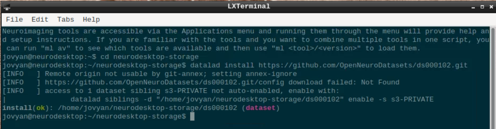
Open a terminal and use datalad to install the dataset:

cd neurodesktop-storage
datalad install https://github.com/OpenNeuroDatasets/ds000102.git

We will use subject 08 as an example here, so we use datalad to download sub-08 and since SPM doesn’t support compressed files, we need to unpack them:

cd ds000102
datalad get sub-08/
gunzip sub-08/anat/sub-08_T1w.nii.gz -f
gunzip sub-08/func/sub-08_task-flanker_run-1_bold.nii.gz -f
gunzip sub-08/func/sub-08_task-flanker_run-2_bold.nii.gz -f
chmod a+rw sub-08/ -R

The task used is described here: https://andysbrainbook.readthedocs.io/en/latest/SPM/SPM_Short_Course/SPM_02_Flanker.html

Starting SPM and visualizing the data

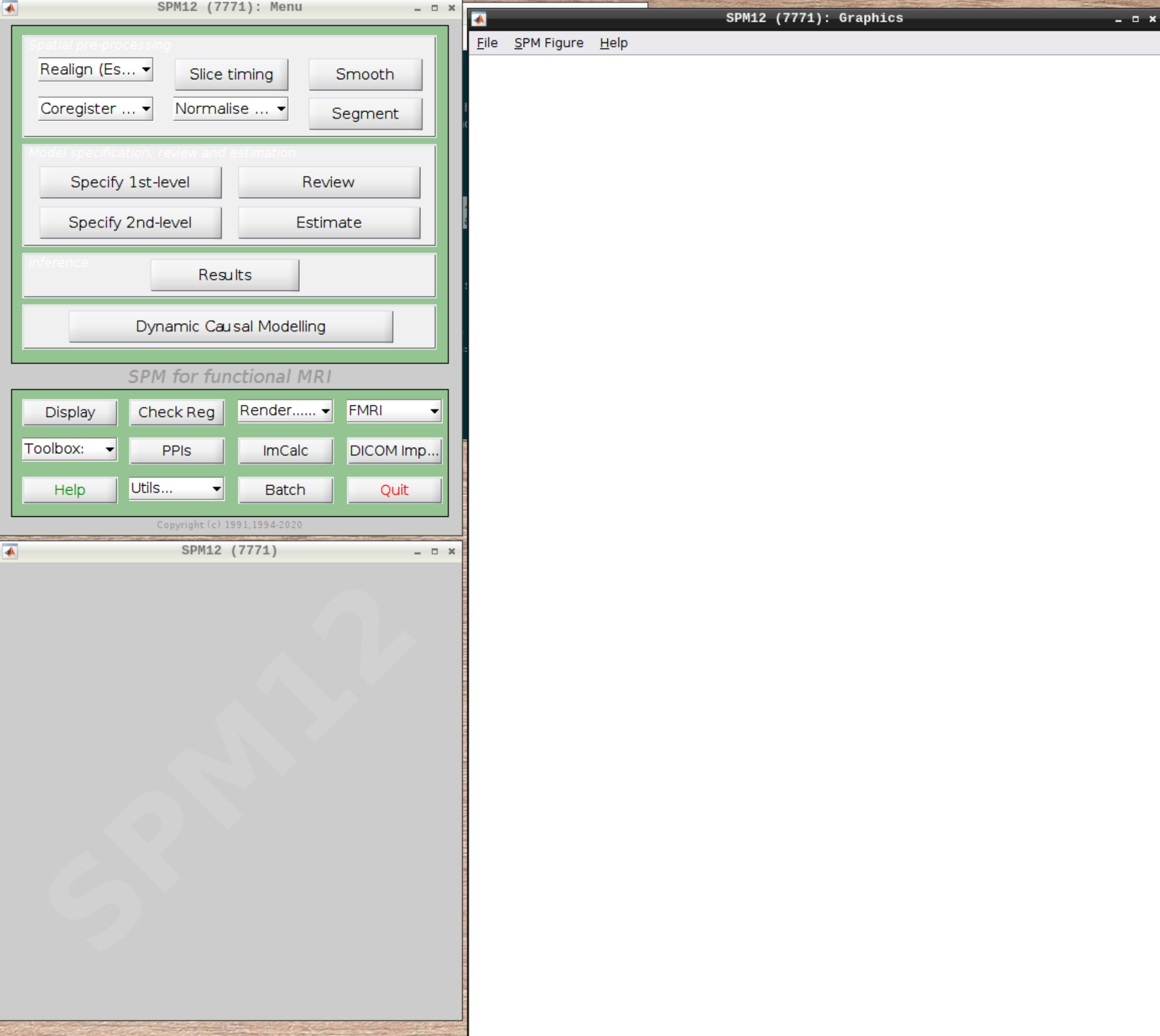
Start spm12GUI from the Application Menu:

When the SPM menu loaded, click on fMRI and the full SPM interface should open up:

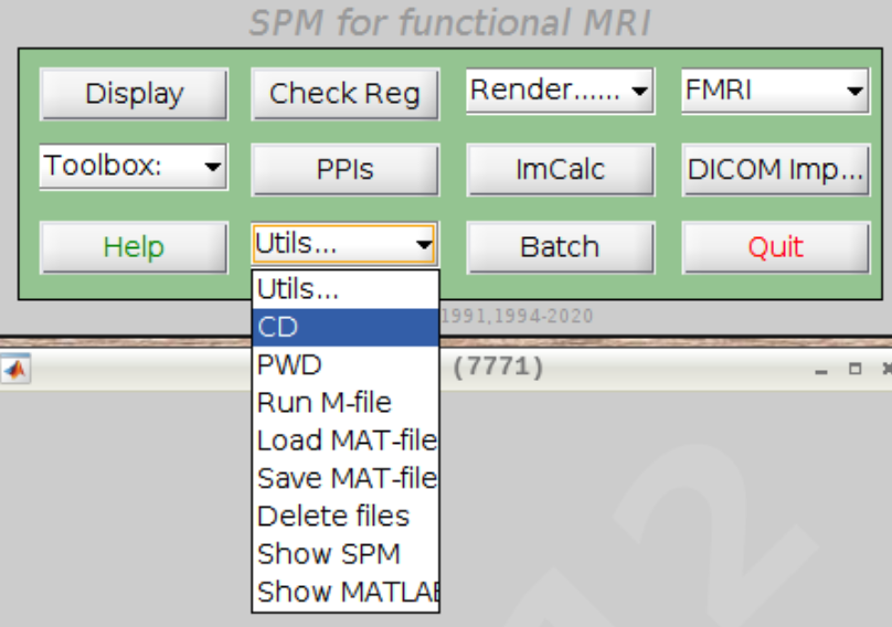
For convenience let’s change our default directory to our example subject. Click on Utils and select CD:

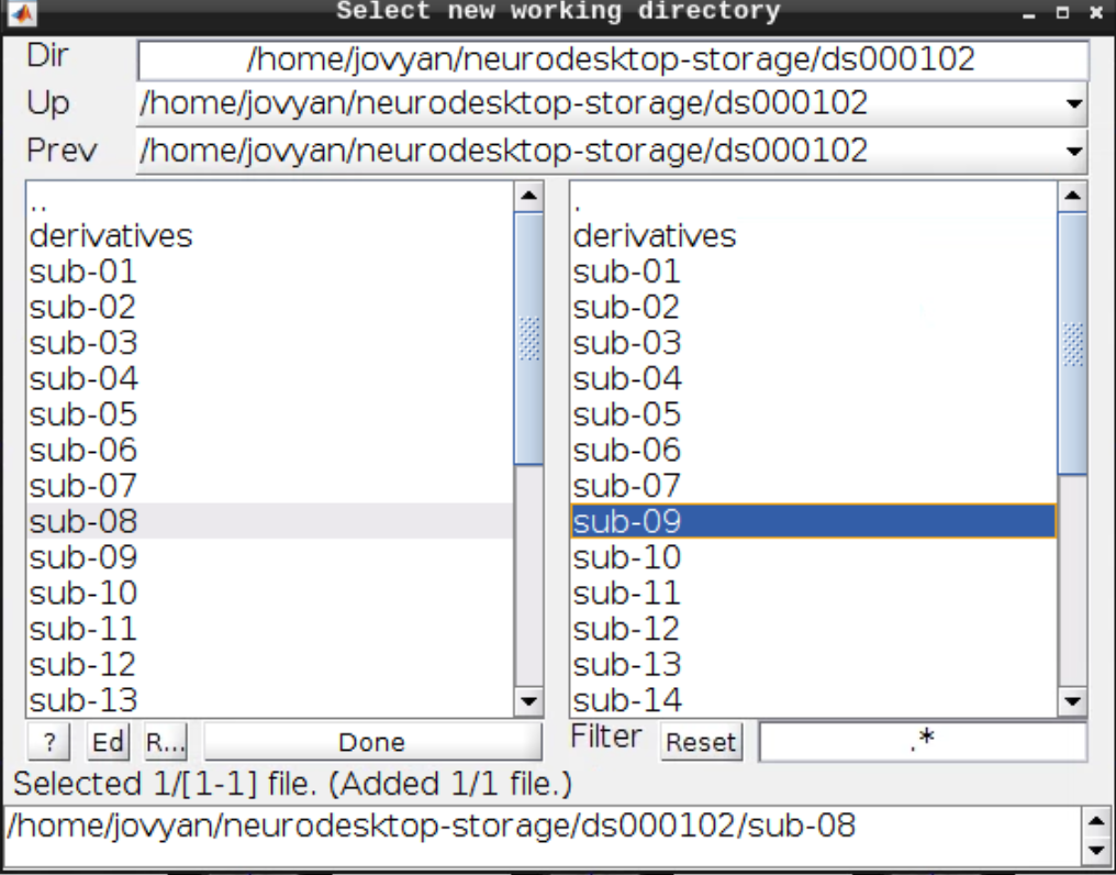
Then navigate to sub-08 and select the directory in the right browser window:

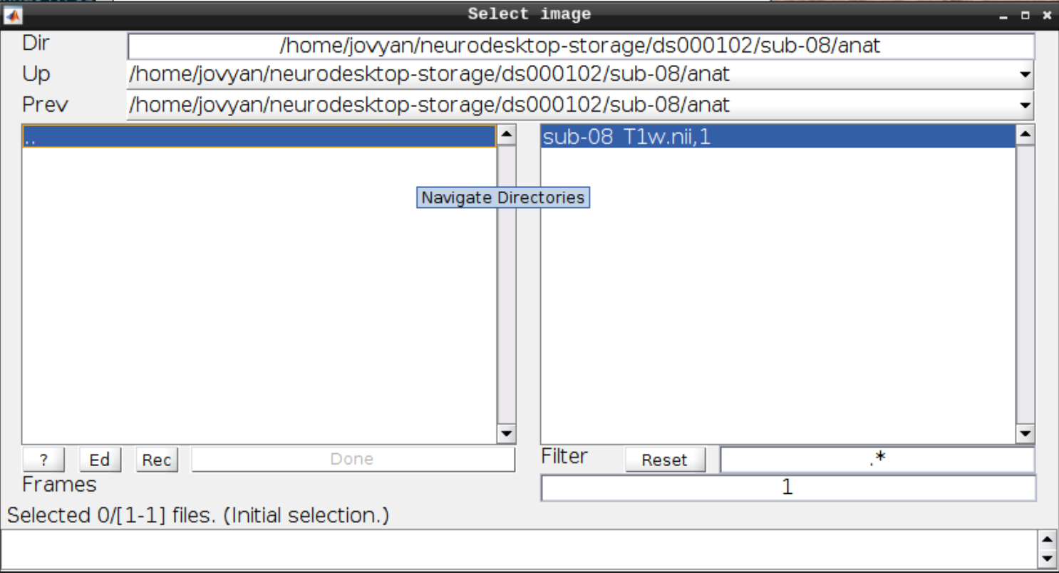
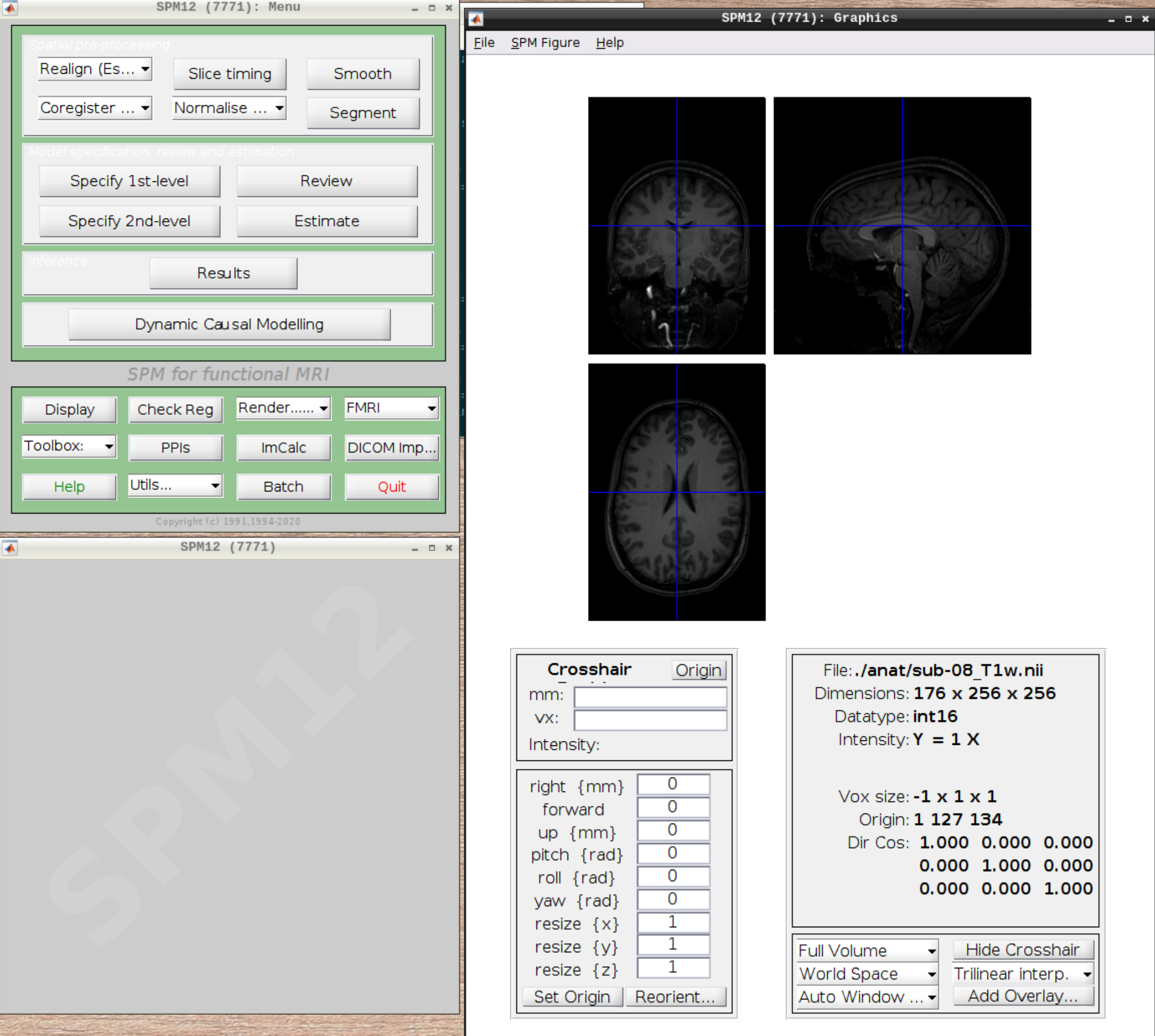
Now let’s visualize the anatomical T1 scan of subject 08 by clicking on Display and navigating and selecting the anatomical scan:

Now let’s look at the functional scans. Use CheckReg and open run-01. Then right click and Browse .... Then set frames to 1:146 and right click Select All

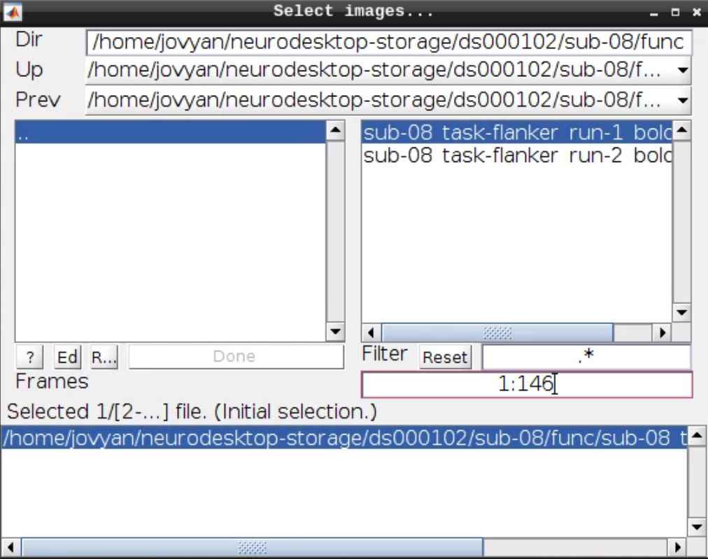
Now we get a slider viewer and we can investigate all functional scans:

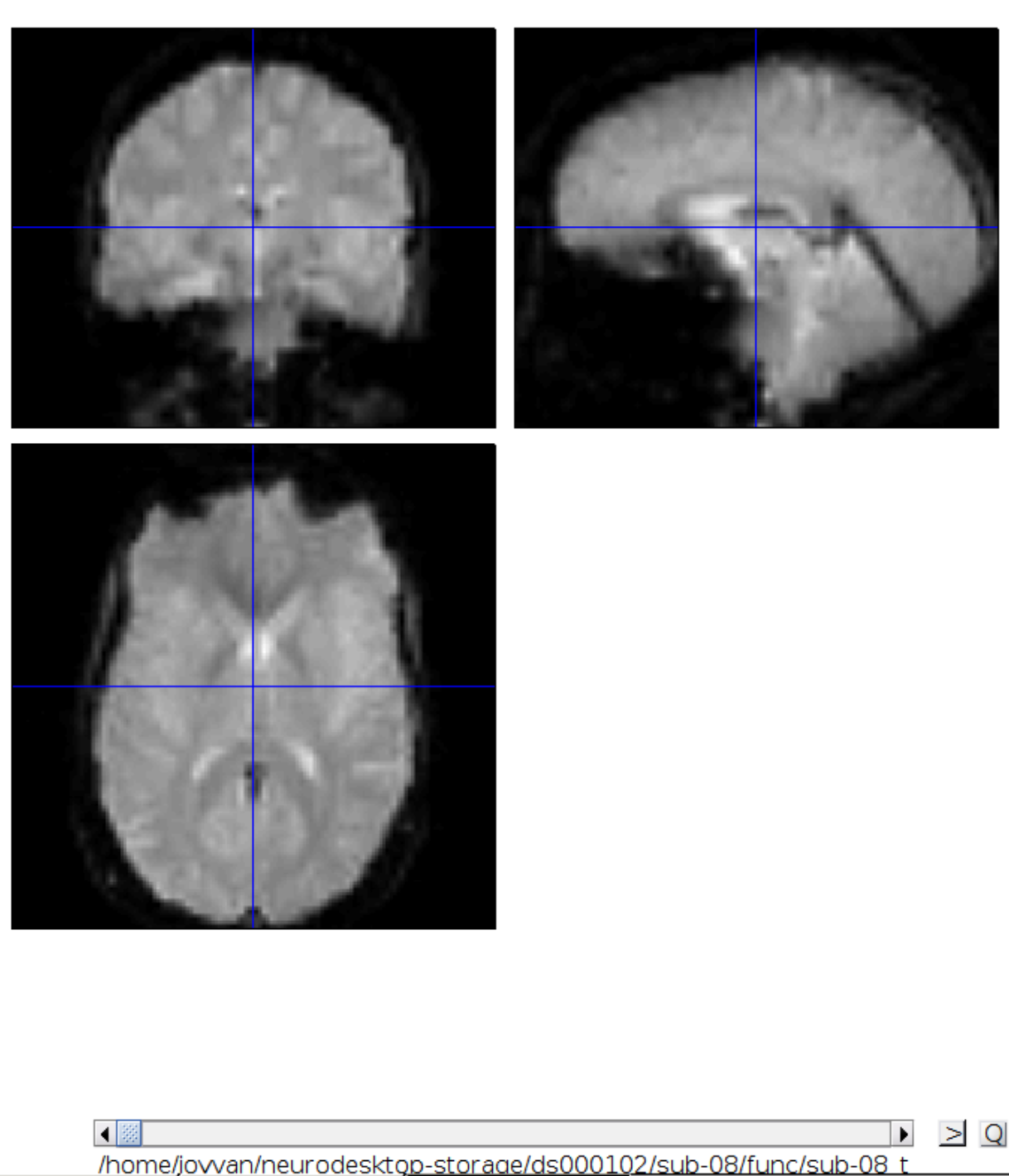
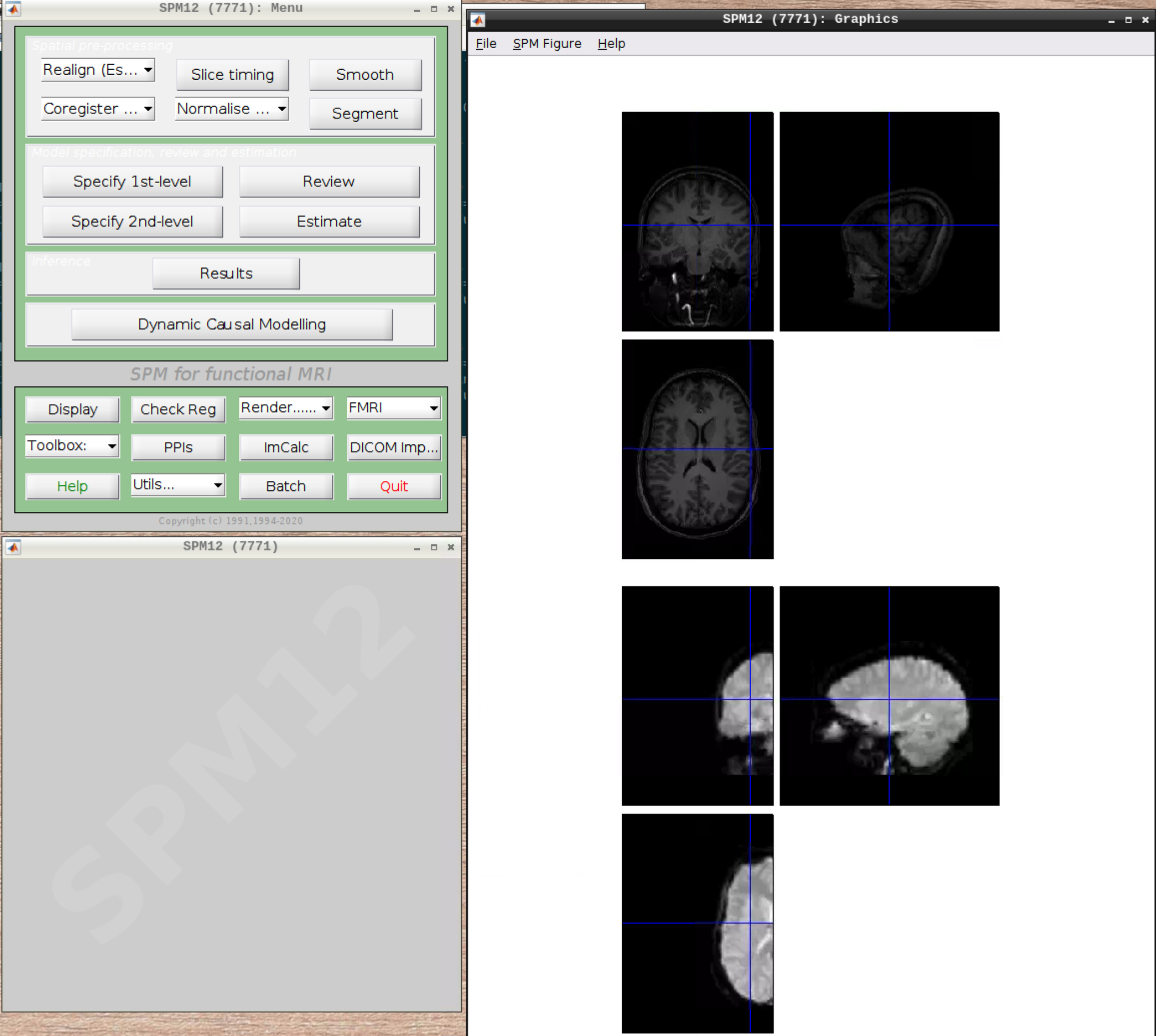
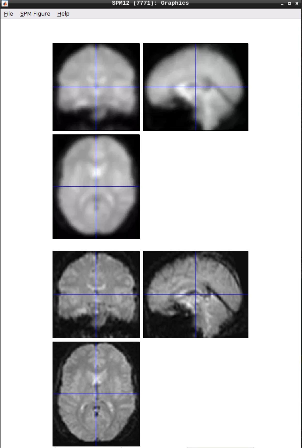
Let’s check the alignment between the anatomical and the functional scans - use CheckReg and open the anatomical and the functional scan. They shouldn’t align yet, because we haven’t done any preprocessing yet:

Preprocessing the data

Realignment

Select Realign (Est & Reslice) from the SPM Menu (the third option):

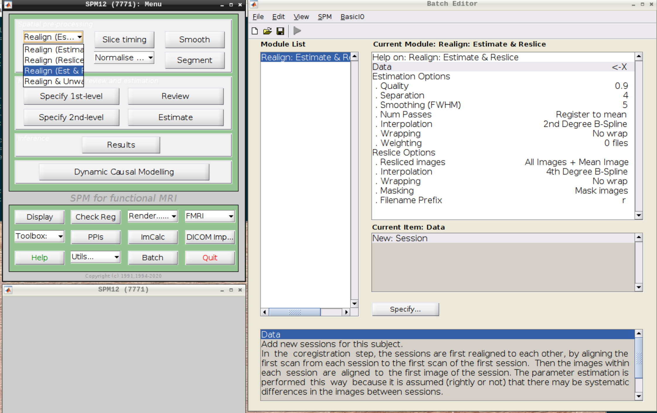
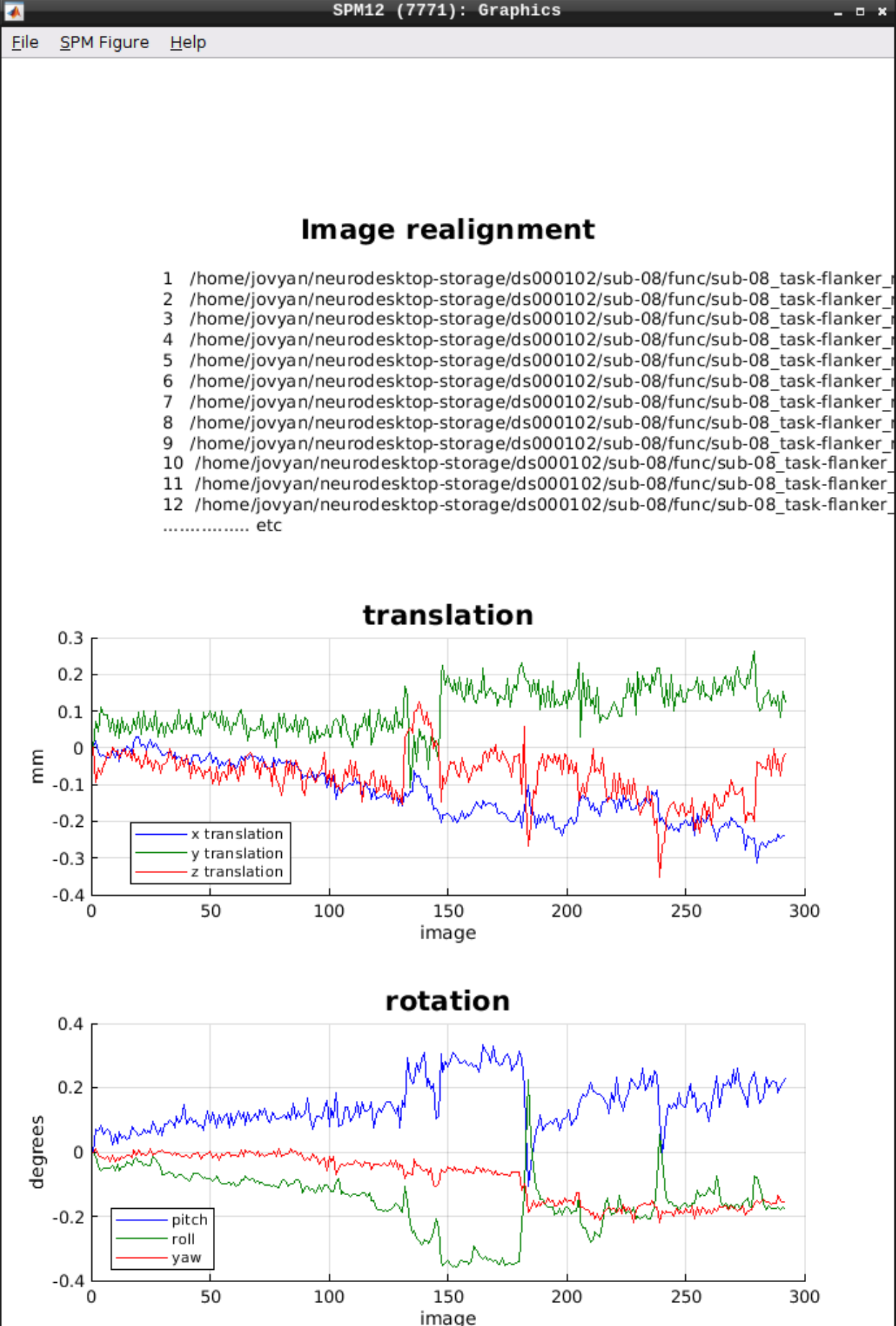
Then select the functional run (important: Select frames from 1:146 again!) and leave everything else as Defaults. Then hit run:

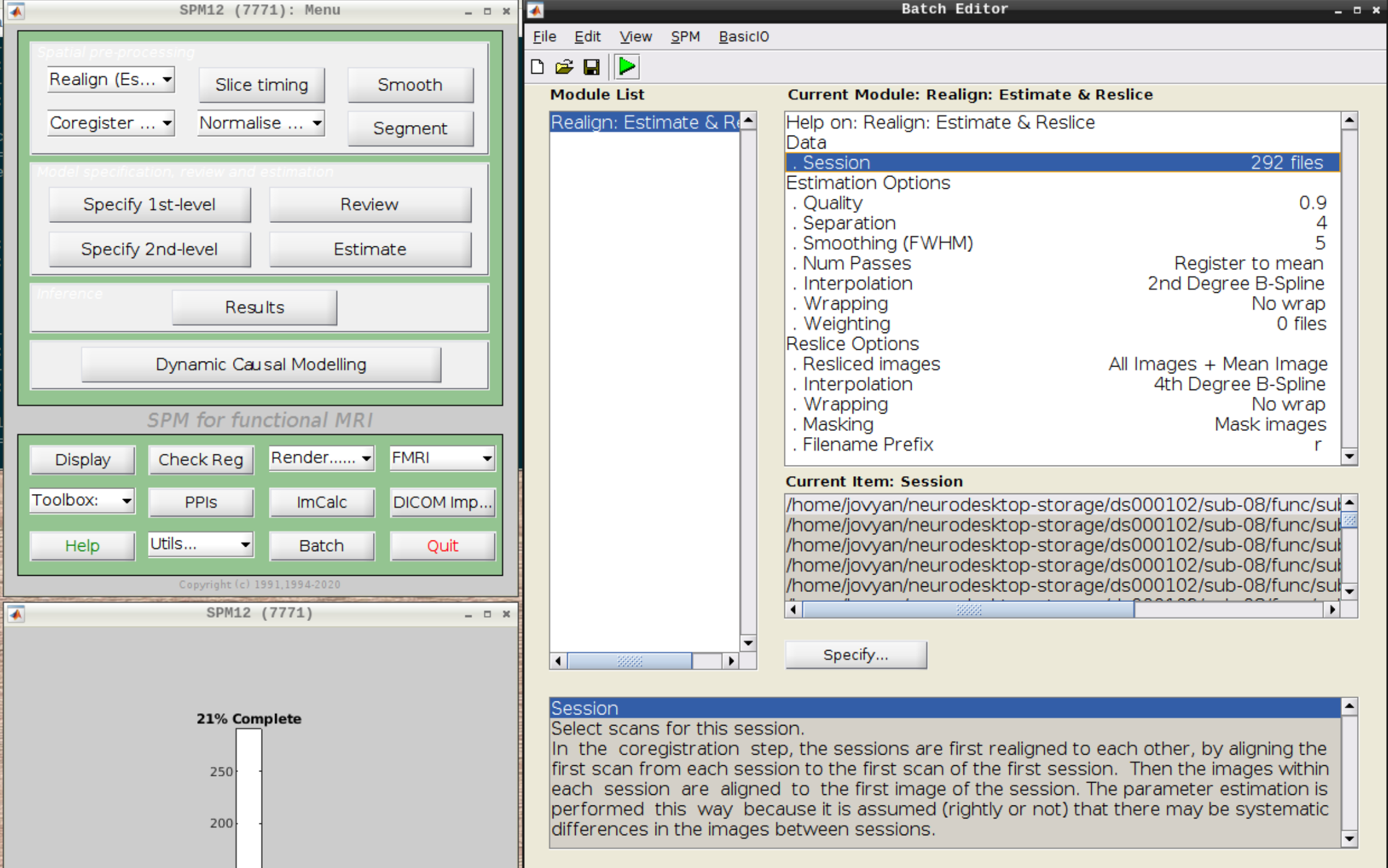
As an output we should see the realignment parameters:

Slice timing correction

Click on Slice timing in the SPM menu to bring up the Slice Timing section in the batch editor:

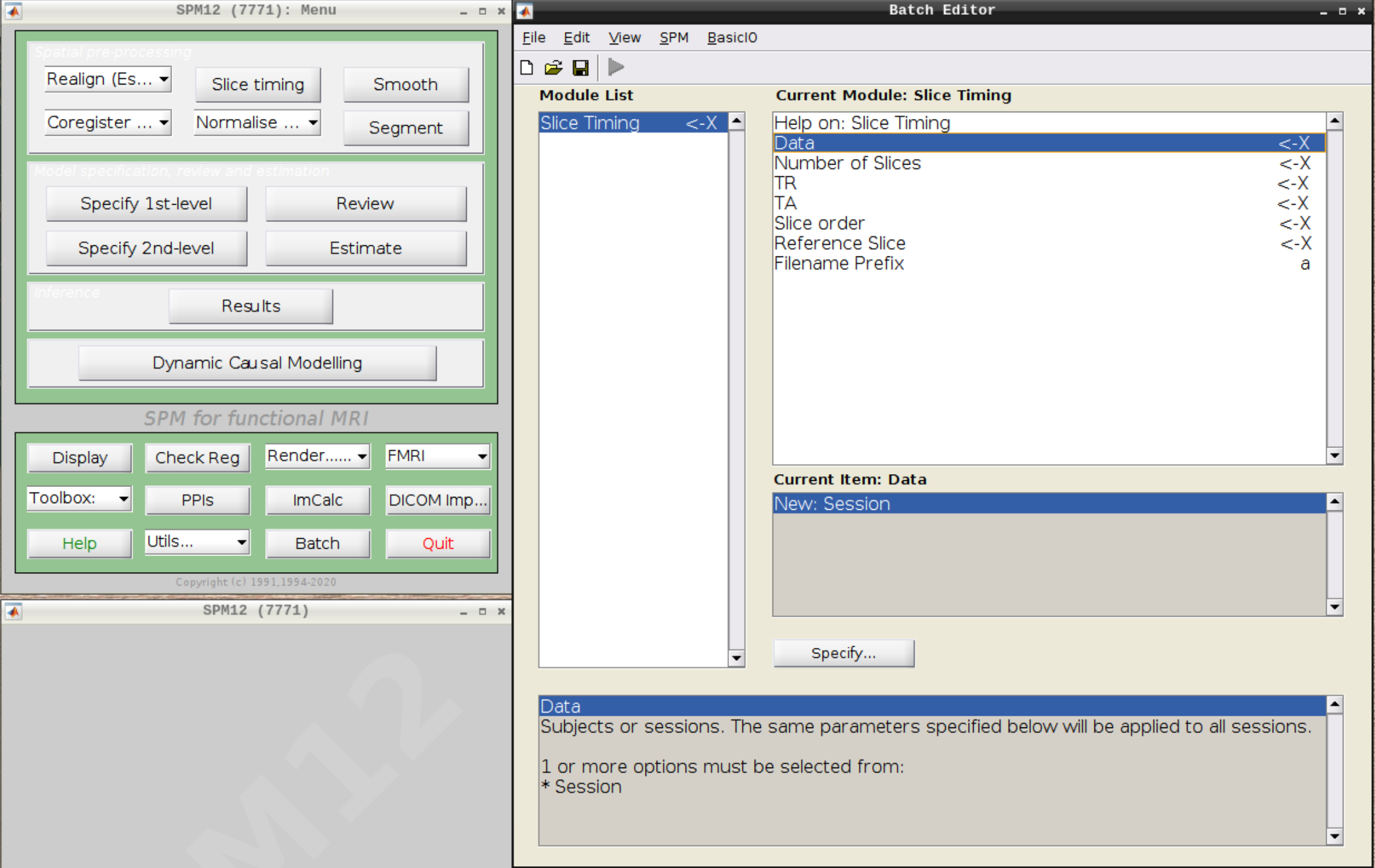
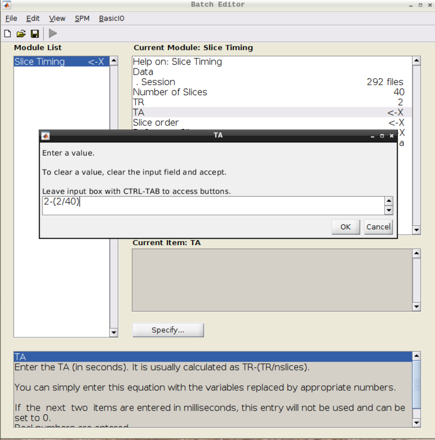
Select the realigned images (use filter rsub and Frames 1:146) and then enter the parameters:

• Number of Slices = 40
• TR = 2
• TA = 1.95
• Slice order = [1:2:40 2:2:40]
• Reference Slice = 1

Coregistration

Now, we coregister the functional scans and the anatomical scan.

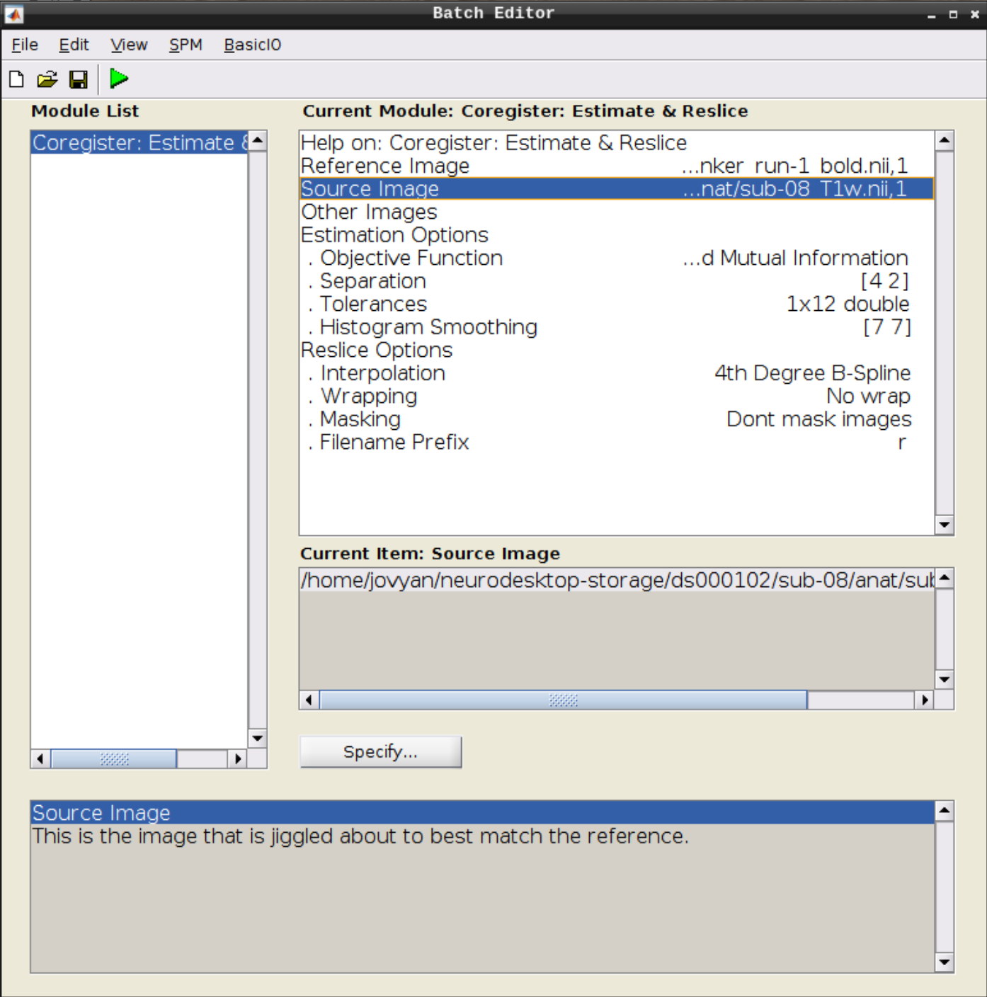
Click on Coregister (Estimate & Reslice) (the third option) in the SPM menu to bring up the batch editor:

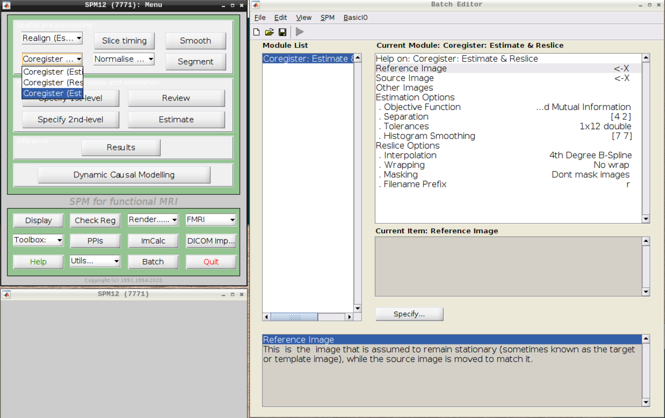
Use the Mean image as the reference and the T1 scan as the source image and hit Play:

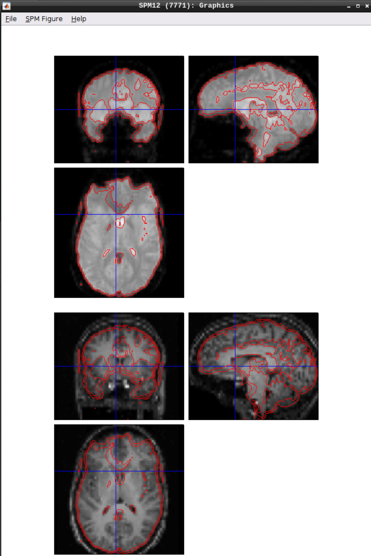
Let’s use CheckReg again and overlay a Contour (Right Click -> Contour -> Display onto -> all) to check the coregistration between the images:

Segmentation

Click the Segmentation button in the SPM menu:

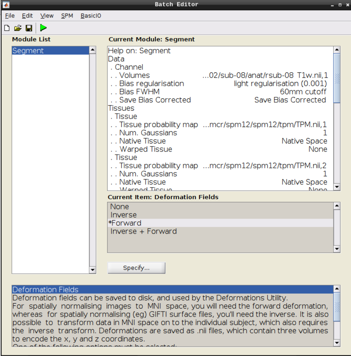
Then change the following settings:

• Volumes = our coregistered anatomical scan rsub-08-T1w.nii
• Save Bias Corrected = Save Bias Correced
• Deformation Fields = Forward

and hit Play again.

Apply normalization

Select Normalize (Write) from the SPM menu:

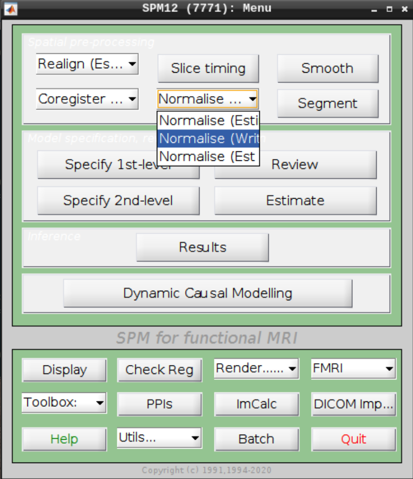
For the Deformation Field select the y_rsub-08 file we created in the last step and for the Images to Write select the arsub-08 functional images (Filter ^ar and Frames 1:146):

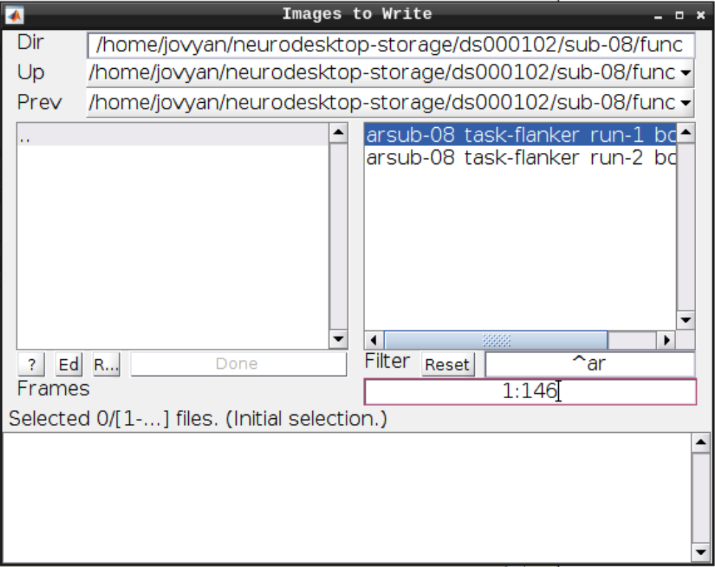
Hit Play again.

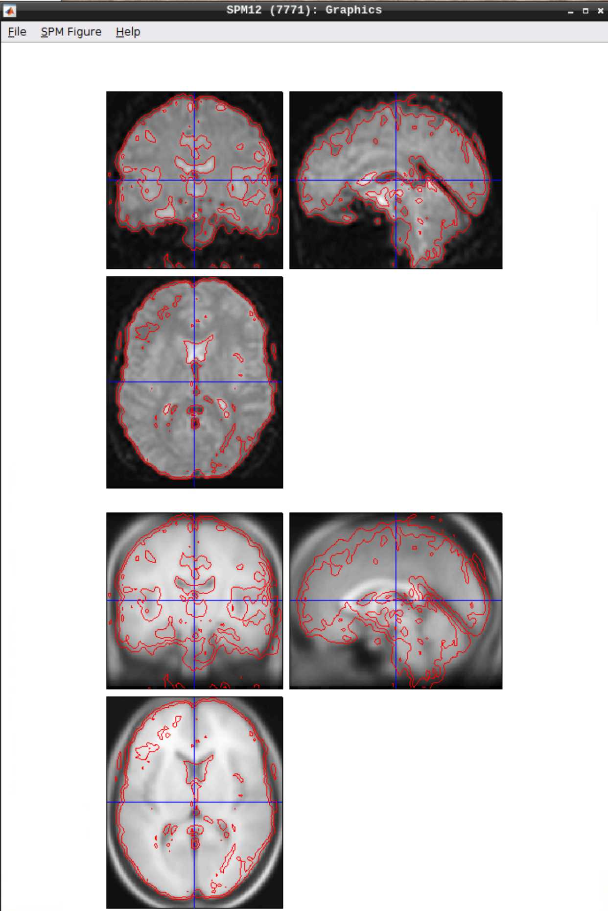
Checking the normalization

Use CheckReg to make sure that the functional scans (starting with w to indicate that they were warped: warsub-08) align with the template (found in /opt/spm12/spm12_mcr/spm12/spm12/canonical/avg305T1.nii):

Smoothing

Click the Smooth button in the SPM menu and select the warped functional scans:

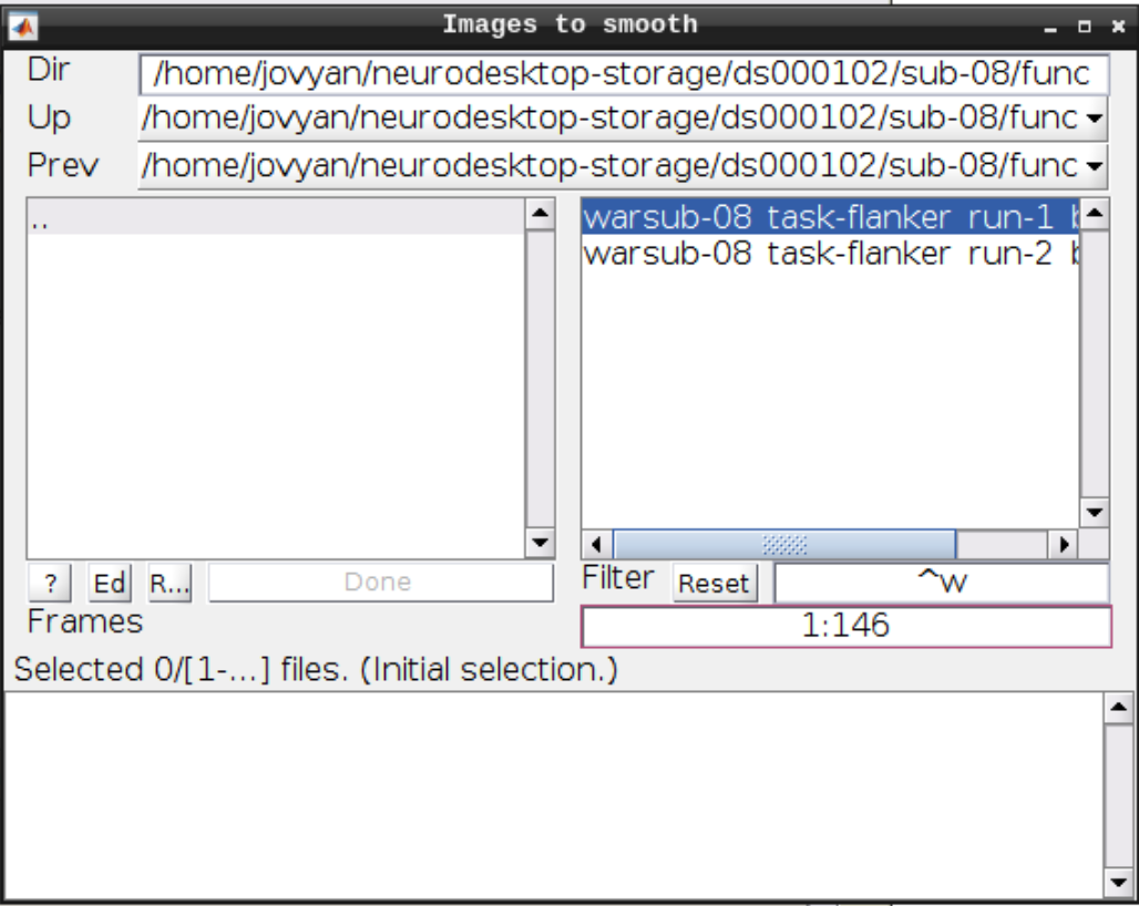
Then click Play.

You can check the smoothing by using CheckReg again:

Analyzing the data

Click on Specify 1st-level - then set the following options:

• Directory: Select the sub-08 top level directory
• Units for design: Seconds
• Interscan interval: 2
• Data & Design: Click twice on New Subject/Session
• Select the smoothed, warped data from run 1 and run 2 for the two sessions respectively
• Create two Conditions per run and set the following:
• For Run 1:
• Name: Inc
• Onsets (you can copy from here and paste with CTRL-V): 0 10 20 52 88 130 144 174 236 248 260 274
• Durations: 2 (SPM will assume that it’s the same for each event)
• Name: Con
• Onsets: 32 42 64 76 102 116 154 164 184 196 208 222
• Durations: 2
• For Run 2:
• Name: Inc
• Onsets: 0 10 52 64 88 150 164 174 184 196 232 260
• Durations: 2
• Name: Con
• Onsets: 20 30 40 76 102 116 130 140 208 220 246 274
• Durations: 2

When done, click the green Play button.

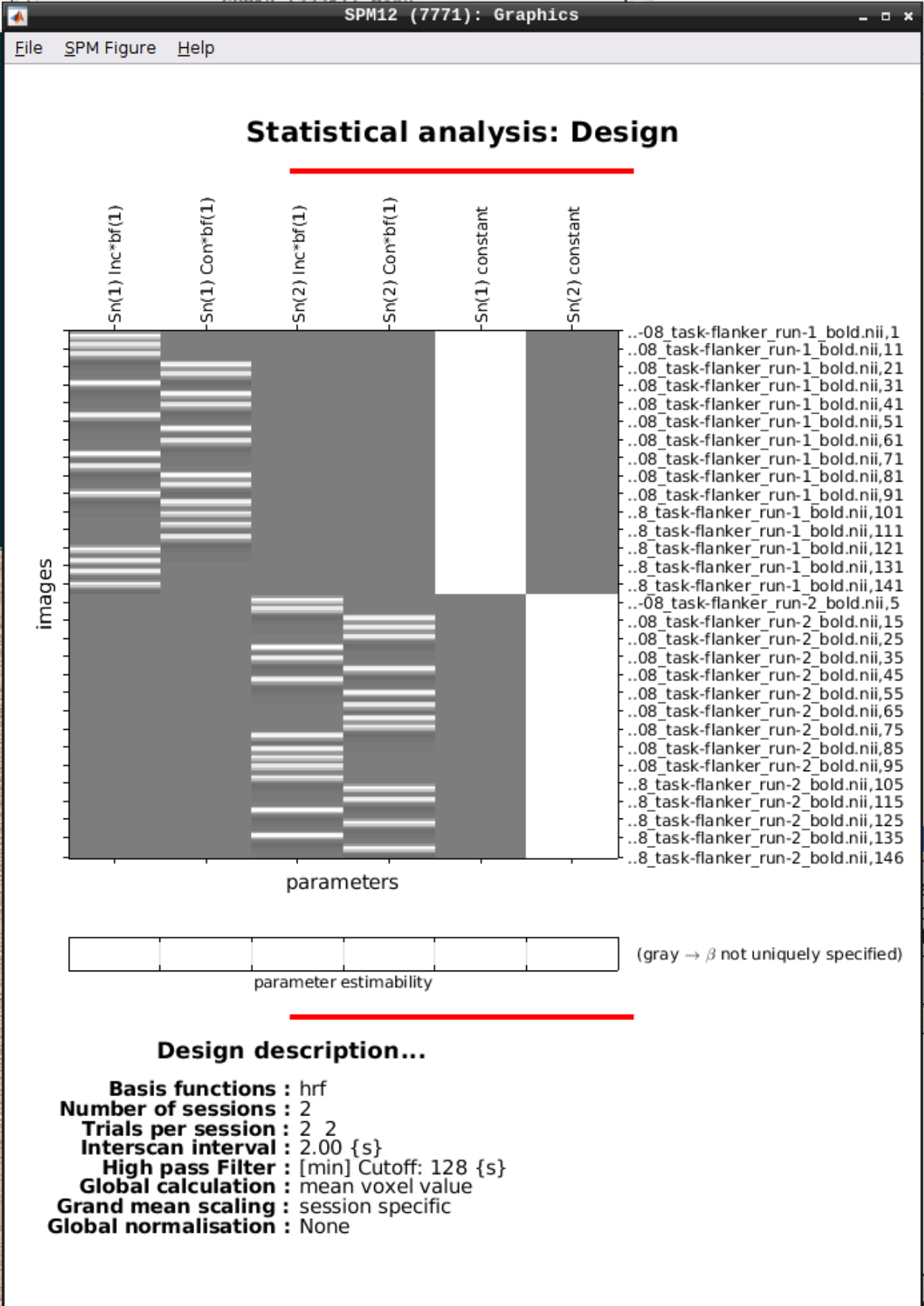
We can Review the design by clicking on Review in the SPM menu and selecting the SPM.mat file in the model directory we specified earlier and it should look like this:

Estimating the model

Click on Estimate in the SPM menu and select the SPM.mat file, then hit the green Play button.

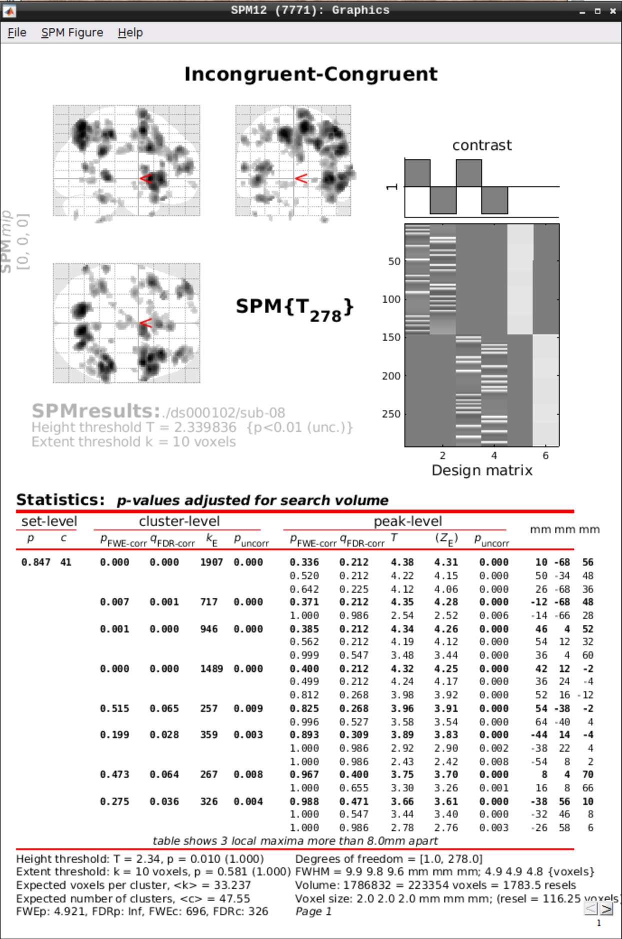
Inference

Now open the Results section and select the SPM.mat file again. Then we can test our hypotheses:

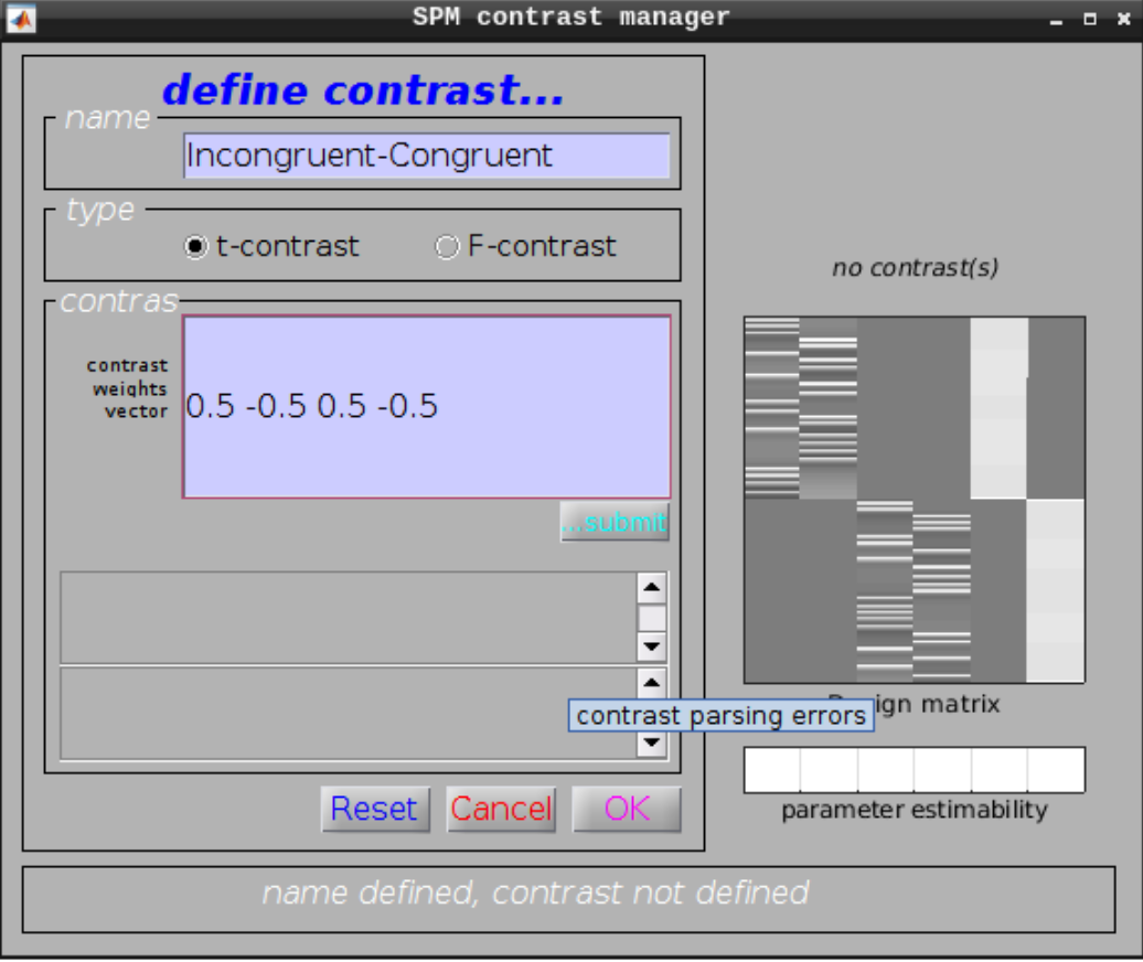
Define a new contrast as:

• Name: Incongruent-Congruent
• Contrast weights vector: 0.5 -0.5 0.5 -0.5

Then we can view the results. Set the following options:

• masking: none”
• p value adjustment to control: Click on “none”, and set the uncorrected p-value to 0.01.
• extent threshold {voxels}: 10