Tutorials & Examples
Tutorials & Examples
1. Understand Neurodesk:
Neurodesk is a flexible and scalable data analysis environment for reproducible neuroimaging. More info
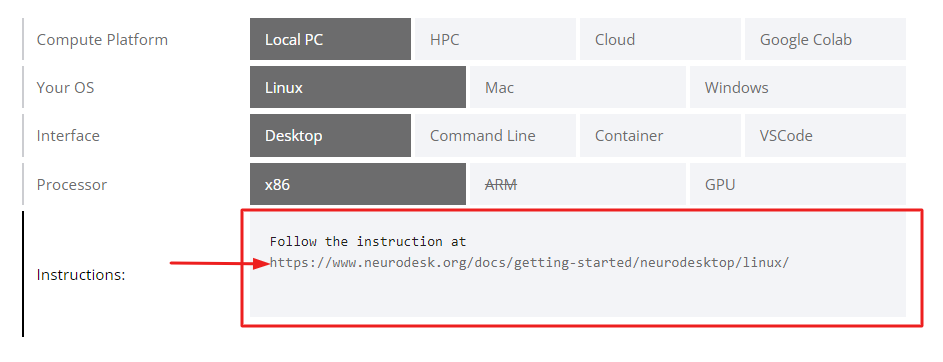
2. Choose Your Setup:
Neurodesk can be used on various platforms including a local PC, High-Performance Computing (HPC), Cloud, and Google Colab. It supports Linux, Mac, and Windows operating systems. You can interact with it through a desktop interface, command line, container, or VSCode. Choose the setup that best suits your needs based on this table.
3. Follow the Instructions:
Once you’ve chosen your setup, follow the instructions provided in the link.
For example, if you’re using Linux on a local PC with a desktop interface, you would follow the instructions at https://www.neurodesk.org/docs/getting-started/neurodesktop/linux/.
4. Video tutorial
See below for a 4-minute tutorial on Installation, Usage and Data Access with Neurodesktop
1 - Examples
Explore the Example Notebooks →
Install Neurodesk and you can load these example notebooks directly in the environment to try them out.
When you install the NeurodeskApp, You can find them under example-notebooks/books.
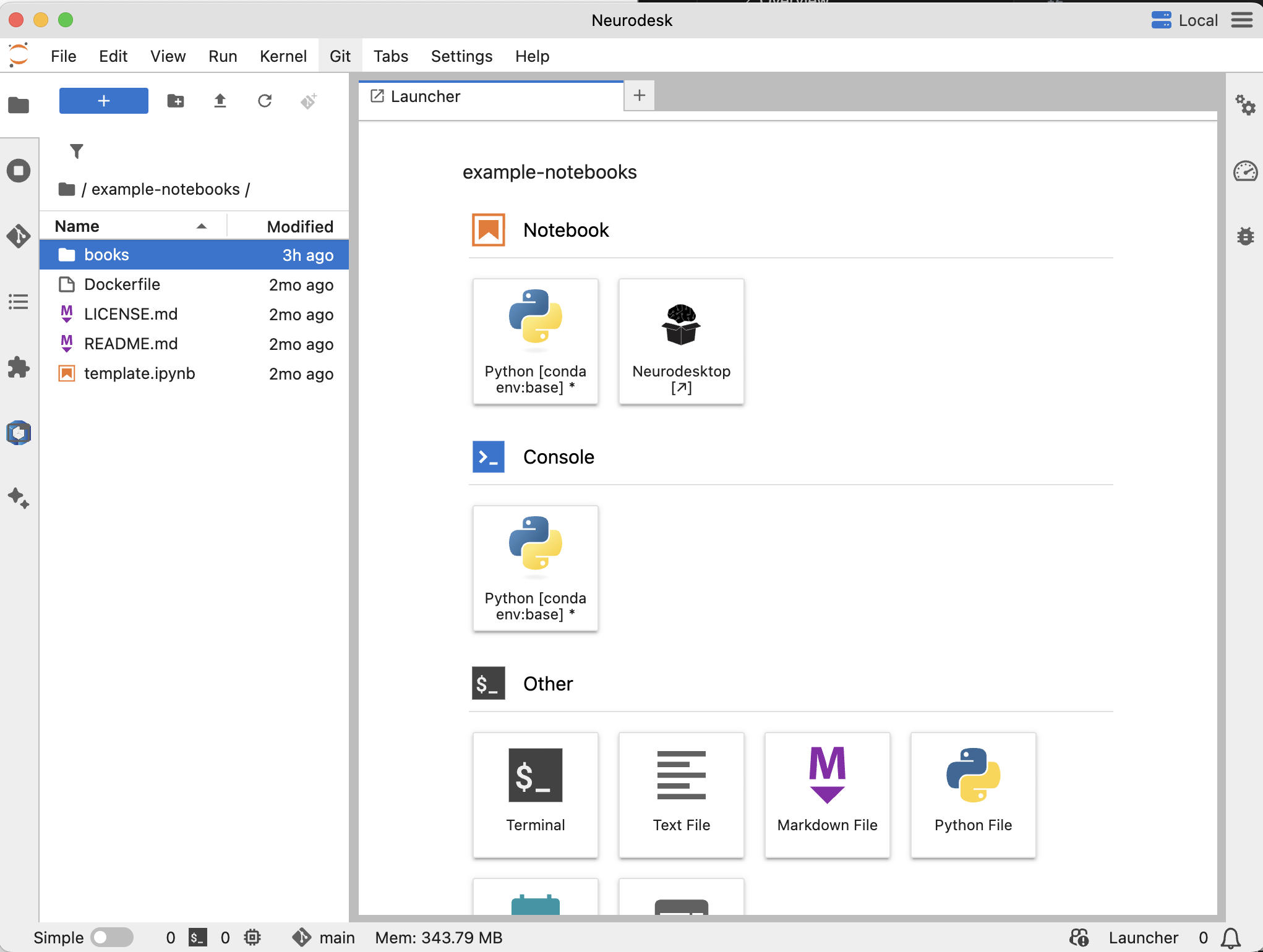
We provide a collection of example Jupyter notebooks to help you get started with Neurodesk and explore its capabilities. These notebooks cover various use cases and analyses.
2.1 - Electrophysiology
Tutorials about processing of EEG/MEG/ECoG data
2.1.1 - Analysing M/EEG Data with FieldTrip
A brief guide to using FieldTrip to analyse electrophysiological data within neurodesk.
This tutorial was created by Judy D Zhu.
Email: judyzhud@gmail.com
Github: @JD-Zhu
Twitter: @JudyDZhu
Getting Setup with Neurodesk
For more information on getting set up with a Neurodesk environment, see herePlease note that this container uses a compiled version of FieldTrip to run scripts (without needing a Matlab license). Code development is not currently supported within the container and needs to be carried out separately in Matlab.
Getting started
- Navigate to Neurodesk->Electrophysiology->fieldtrip->fieldtrip20211114 in the menu:

Once this window is loaded, you are ready to go:

- Type the following into the command window (replacing “./yourscript.m” with the name of your custom script - if the script is in the current folder, use “./” before the script name like in the example; otherwise, please supply the full path):
run_fieldtrip.sh /opt/MCR/v99 ./yourscript.m
For example, here we ran a script to browse some raw data:

The fieldtrip GUI is displayed automatically and functions as it normally would when running inside Matlab.
NOTES:
- The script can only call FieldTrip and SPM functions (these are the only functions in the search path, and the search path cannot be altered using addpath)
- The script cannot include internal functions
- The script can use all the MATLAB toolboxes included in the compiled version of FieldTrip
2.1.2 - Analysing EEG Data with MNE
Use mne-python to load, pre-process, and plot example EEG data in a jupyter notebook through vscode.
This tutorial was created by Angela Renton.
Github: @air2310
Getting Setup with Neurodesk
For more information on getting set up with a Neurodesk environment, see hereGetting started
To begin, navigate to Neurodesk->Electrophysiology->mne->vscodeGUI 0.23.4 in the menu. This version of vscode has been installed in a software container together with the a conda environment containing MNE-python. Note that if you open any other version of vscode in Neurodesk, you will not be able to access the MNE conda environment.


Open the folder: “/home/user/Desktop/storage” or a subfolder in which you would like to store this demo. In this folder, create a new file named “EEGDemo.ipynb” or something similar:

If this is your first time opening a Jupyter notebook on vscode in neurodesktop, you may see the following popup. If so, click “install” to install the vscode extensions for Jupyter.

Select MNE python kernel
Next, we need to direct vscode to use the python kernel associated with MNE. In the top right corner of your empty jupyter notebook, click “Select Kernel”:

Then, select mne-0.23.4 from the dropdown menu, which should look something like this:

Activate the MNE conda environment in the terminal
Next, we’ll activate the same MNE environment in a terminal. From the top menu in vscode, select Terminal->New Terminal, or hit [Ctrl]+[Shift]+[`].
If this is your first time using vscode in this container, you may have to initialise conda by typing conda init bash in the bash terminal. After initialising bash, you will have to close and then reopen the terminal.
Once you have initialised conda, you can activate the MNE environment in the terminal:
conda activate mne-0.23.4
You should now see “(mne-0.23.4)” ahead of the current line in the terminal.
Download sample data
In the terminal (in which you have activated the MNE environment), input the following code to download some BIDS formatted sample EEG data:
Remember to update the path to the location you are storing this tutorial!
pip install osfclient
osf -p C689U fetch Data_sample.zip /neurodesktop-storage/EEGDEMO/Data_sample.zip
unzip Data_sample.zip
This is a small dataset with only 5 EEG channels from a single participant. The participant is viewing a frequency tagged display and is cued to attend to dots tagged at one frequency or another (6 Hz, 7.5 Hz) for long, 15 s trials. To read more about the dataset, click here
Plotting settings
To make sure our plots retain their interactivity, set the following line at the top of your notebook:
This will mean your figures pop out as individual, interactive plots that will allow you to explore the data, rather than as static, inline plots. You can switch “qt” to “inline” to switch back to default, inline plotting.
Loading and processing data
NOTE: MNE has many helpful tutorials which delve into data processing and analysis using MNE-python in much further detail. These can be found here
Begin by importing the necessary modules and creating a pointer to the data:
# Interactive plotting
%matplotlib qt

# Import modules
import os
import numpy as np
import mne

# Load data
sample_data_folder = '/neurodesktop-storage/EEGDemo/Data_sample'
sample_data_raw_file = os.path.join(sample_data_folder, 'sub-01', 'eeg',
                                    'sub-01_task-FeatAttnDec_eeg.vhdr')
raw = mne.io.read_raw_brainvision(sample_data_raw_file , preload=True)
the raw.info structure contains information about the dataset:
# Display data info
print(raw)
print(raw.info)
This data file did not include a montage. Lets create one using standard values for the electrodes we have:
# Create montage
montage = {'Iz':  [0, -110, -40],
            'Oz': [0, -105, -15],
            'POz': [0,   -100, 15],
            'O1': [-40, -106, -15],
            'O2':  [40, -106, -15],
 }

montageuse = mne.channels.make_dig_montage(ch_pos=montage, lpa=[-82.5, -19.2, -46], nasion=[0, 83.2, -38.3], rpa=[82.2, -19.2, -46]) # based on mne help file on setting 10-20 montage
Next, lets visualise the data.
This should open an interactive window in which you can scroll through the data. See the MNE documentation for help on how to customise this plot.

If, upon visual inspection, you decide to exclude one of the channels, you can specify this in raw.info[‘bads’] now. For example:
raw.info['bads'] = ['POz']
Next, we’ll extract our events. The trigger channel in this file is incorrectly scaled, so we’ll correct that before we extract our events:
# Correct trigger scaling
trigchan = raw.copy()
trigchan = trigchan.pick('TRIG')
trigchan._data = trigchan._data*1000000

# Extract events
events = mne.find_events(trigchan, stim_channel='TRIG', consecutive=True, initial_event=True, verbose=True)
print('Found %s events, first five:' % len(events))
print(events[:5])

# Plot events
mne.viz.plot_events(events, raw.info['sfreq'], raw.first_samp)

Now that we’ve extracted our events, we can extract our EEG channels and do some simple pre-processing:
# select
eeg_data = raw.copy().pick_types(eeg=True, exclude=['TRIG'])

# Set montage
eeg_data.info.set_montage(montageuse)

# Interpolate
eeg_data_interp = eeg_data.copy().interpolate_bads(reset_bads=True)

# Filter Data
eeg_data_interp.filter(l_freq=1, h_freq=45, h_trans_bandwidth=0.1)
Let’s visualise our data again now that it’s cleaner:
#plot results again, this time with some events and scaling.
eeg_data_interp.plot(events=events, duration=10.0, scalings=dict(eeg=0.00005), color='k', event_color='r')

That’s looking good! We can even see hints of the frequency tagging. It’s about time to epoch our data.
# Epoch to events of interest
event_id = {'attend 6Hz K': 23, 'attend 7.5Hz K':  27}

# Extract 15 s epochs relative to events, baseline correct, linear detrend, and reject
# epochs where eeg amplitude is > 400
epochs = mne.Epochs(eeg_data_interp, events, event_id=event_id, tmin=0,
                    tmax=15, baseline=(0, 0), reject=dict(eeg=0.000400), detrend=1)

# Drop bad trials
epochs.drop_bad()
We can average these epochs to form Event Related Potentials (ERPs):
# Average erpochs to form ERPs
attend6 = epochs['attend 6Hz K'].average()
attend75 = epochs['attend 7.5Hz K'].average()

# Plot ERPs
evokeds = dict(attend6=list(epochs['attend 6Hz K'].iter_evoked()),
               attend75=list(epochs['attend 7.5Hz K'].iter_evoked()))
mne.viz.plot_compare_evokeds(evokeds, combine='mean')

In this plot, we can see that the data are frequency tagged. While these data were collected, the participant was performing an attention task in which two visual stimuli were flickering at 6 Hz and 7.5 Hz respectively. On each trial the participant was cued to monitor one of these two stimuli for brief bursts of motion. From previous research, we expect that the steady-state visual evoked potential (SSVEP) should be larger at the attended frequency than the unattended frequency. Lets check if this is true.
We’ll begin by exporting our epoched EEG data to a numpy array
# Preallocate
n_samples = attend6.data.shape[1]
sampling_freq = 1200 # sampling frequency
epochs_np = np.empty((n_samples, 2) )

# Get data - averaging across EEG channels
epochs_np[:,0] = attend6.data.mean(axis=0)
epochs_np[:,1] = attend75.data.mean(axis=0)
Next, we can use a Fast Fourier Transform (FFT) to transform the data from the time domain to the frequency domain. For this, we’ll need to import the FFT packages from scipy:
from scipy.fft import fft, fftfreq, fftshift

# Get FFT
fftdat = np.abs(fft(epochs_np, axis=0)) / n_samples
freq = fftfreq(n_samples, d=1 / sampling_freq)  # get frequency bins
Now that we have our frequency transformed data, we can plot our two conditions to assess whether attention altered the SSVEP amplitudes:
import matplotlib.pyplot as plt

fig,ax = plt.subplots(1, 1)

ax.plot(freq, fftdat[:,0], '-', label='attend 6Hz', color=[78 / 255, 185 / 255, 159 / 255])
ax.plot(freq, fftdat[:,1], '-', label='attend 7.5Hz', color=[236 / 255, 85 / 255, 58 / 255])
ax.set_xlim(4, 17)
ax.set_ylim(0, 1e-6)
ax.set_title('Frequency Spectrum')
ax.legend()

This plot shows that the SSVEPs were indeed modulated by attention in the direction we would expect! Congratulations! You’ve run your first analysis of EEG data in neurodesktop.
2.2 - Functional Imaging
Tutorials about processing functional MRI data
2.2.1 - Connectome Workbench
A tutorial for accessing and visualizing the 7T HCP Retinotopy Dataset on Connectome Workbench.
This tutorial was created by Fernanda L. Ribeiro.
Email: fernanda.ribeiro@uq.edu.au
Github: @felenitaribeiro
Twitter: @NandaRibeiro93
This tutorial documents how to use Connectome Workbench on NeuroDesk for visualizing the 7T HCP Retinotopy Dataset.
Getting Setup with Neurodesk
For more information on getting set up with a Neurodesk environment, see hereDownload data
First, make sure you register for the Human Connectome Project Open Access Data: https://www.humanconnectome.org/study/hcp-young-adult/data-use-terms
Register to the BALSA database: https://balsa.wustl.edu/.

- Login and download the scene files containing the retinotopic maps available at: https://balsa.wustl.edu/study/9Zkk.

These files include preprocessed collated data from 181 participants, including retinotopic, curvature, midthickness, and myelin maps.
- Finally, unzip the S1200_7T_Retinotopy_9Zkk.zip file.

Visualizing scene files
Using Connectome Workbench, you can load “.scene” files and visualize all individuals’ retinotopic maps.
To do so, follow the next steps:
- In the application menu, navigate to Neurodesk → functional imaging → connectomeworkbench → connectomeworkbench 1.5.0

- On the terminal shell that pops up, type in:

- Click on “Open Other”

and search for a scene file

in the path where your data is

Finally, select the desired file and open it:

- On the ‘Scenes’ window that will pop up, select the first option.

The default images are the average maps.

- To change the displayed images for an individual’s data instead, click on the first ticked dropdown menu

and select “S1200_7T_Retinotopy181.All.Fit1_PolarAngle_MSMALL.32k_fs_LR.dscalar.nii”:

- Now, you should be able to select specific maps from the dropdown menu on the right. For example, here we have the first individual polar angle map (top left):

Now we have the fifth:

- You can do the same for the other functional maps by navigating through the tabs at the top.

2.2.2 - Using fmriprep with neurodesk on an HPC
A brief guide to using fmriprep with neurodesk
This tutorial was created by Kelly G. Garner.
Github: @kel_github
This workflow documents how to use fmriprep with neurodesk and provides some details that may help you troubleshoot some common problems I found along the way.
Getting Setup with Neurodesk
For more information on getting set up with a Neurodesk environment, see hereAn example notebook can be found here:
https://github.com/NeuroDesk/example-notebooks/blob/main/books/functional_imaging/fmriprep.ipynb
Assumptions
Steps
Launch Neurodesk
From the launcher, click the Neurodesktop icon:

Open fmriprep
Now you’re in Neurodesk, use the menus to first open the neurodesk options

and then select fMRIPrep. Note that the latest version will be the lowest on the dropdown list:

This will open a terminal window where fMRIPrep is ready and waiting at your fingertips - woohoo!

Setting up fmriprep command
You can now enter your fmriprep command straight into the command line in the newly opened terminal. Here is a quick guide to the command I have used with the options I have found most useful. Note that fMRIPrep requests the path to the freesurfer license file, which should be somewhere in your system for neurodesk to read - e.g. in ’neurodesktop-storage'.
export ITK_GLOBAL_DEFAULT_NUMBER_OF_THREADS=6 # specify the number of threads you want to use

fmriprep /path/to/your/data \ # this is the top level of your data folder
         /path/to/your/data/derivatives \ # where you want fmriprep output to be saved
         participant \ # this tells fmriprep to analyse at the participant level
         --fs-license-file /path/to/your/freesurfer.txt \ # where the freesurfer license file is
         --output-spaces T1w MNI152NLin2009cAsym fsaverage fsnative \
         --participant-label 01 \ # put what ever participant labels you want to analyse
         --nprocs 6 --mem 10000 \ # fmriprep can be greedy on the hpc, make sure it is not
         --skip_bids_validation \ # its normally fine to skip this but do make sure your data are BIDS enough
         -v # be verbal fmriprep, tell me what you are doing
Then hit return and fMRIPrep should now be merrily working away on your data :)
Some common pitfalls I have learned from my mistakes (and sometimes from others)
If fmriprep hangs it could well be that you are out of disk space. Sometimes this is because fmriprep created a work directory in your home folder which is often limited on the HPC. Make sure fmriprep knows to use a work drectory in your scratch. you can specify this in the fmriprep command by using -w /path/to/the/work/directory/you/made
I learned the following from TomCat (@thomshaw92) - fMRIPrep can get confused between subjects when run in parallel. Parallelise with caution.
If running on a HPC, make sure to set the processor and memory limits, if not your job will get killed because it hogs all the resources.
2.2.3 - Using mriqc with neurodesk on HPC
A brief guide to using mriqc with neurodesk.
This tutorial was created by Kelly G. Garner.
Github: @kel_github
This workflow documents how to use MRIQC with neurodesk and provides some details that may help you troubleshoot some common problems I found along the way.
Getting Setup with Neurodesk
For more information on getting set up with a Neurodesk environment, see here
Assumptions
NOTE: MRIQC has its $HOME variable hardcoded to be /home/mriqc. This leads to problems on some HPCs. A workaround is to run this before mriqc:
export neurodesk_singularity_opts="--home $HOME:/home"
Steps
Launch Neurodesk
From the launcher, click the Neurodesktop icon:

Open MRIQC
Now you’re in Neurodesk, use the menus to first open the neurodesk options

and then select MRIQC. Note that the latest version will be the lowest on the dropdown list:

This will open a terminal window where MRIQC is ready and waiting at your fingertips - woohoo!

Setting up mriqc command
You can now enter the following mriqc commands straight into the command line in the newly opened terminal window.
export ITK_GLOBAL_DEFAULT_NUMBER_OF_THREADS=6 # specify the number of threads you want to use

mriqc /path/to/your/data \ # this is the top level of your data folder
         /path/to/your/data/derivatives \ # where you want mriqc output to be saved
         participant \ # this tells mriqc to analyse at the participant level
         --participant-label 01 \ # put what ever participant labels you want to analyse
         --work-dir /path/to/work/directory \ #useful to specify so your home directory definitely does not get clogged
         --nprocs 6 --mem_gb 10000 \ # mriqc can be greedy on the hpc, make sure it is not
         -v # be verbal mriqc, tell me what you are doing
Note that above I have set the processor and memory limits. This is because I was in this case running on an HPC, and I used those commands to stop MRIQC from hogging all the resources. You may want to skip those inputs if you’re running MRIQC locally.
OR: if you have run all the participants and you just want the group level report, use these mriqc commands instead:
mriqc /path/to/your/data \ # this is the top level of your data folder
         /path/to/your/data/derivatives \ # where you want mriqc output to be saved. As you are running the group level analysis this folder should be prepopulated with the results of the participant level analysis
         group \ # this tells mriqc to agive you the group report
         -w /path/to/work/directory \ #useful to specify so your home directory definitely does not get clogged
         --nprocs 6 --mem_gb 10000 \ # mriqc can be greedy on the hpc, make sure it is not
         -v # be verbal mriqc, tell me what you are doing
Hit enter, and mriqc should now be merrily working away on your data :)
2.2.4 - PhysIO
Example workflow for the PhysIO Toolbox
This tutorial was created by Lars Kasper.
Github: @mrikasper
Twitter: @mrikasper
Getting Setup with Neurodesk
For more information on getting set up with a Neurodesk environment, see hereOrigin
The PhysIO Toolbox implements ideas for robust physiological noise modeling in fMRI, outlined in this paper:
- Kasper, L., Bollmann, S., Diaconescu, A.O., Hutton, C., Heinzle, J., Iglesias,
S., Hauser, T.U., Sebold, M., Manjaly, Z.-M., Pruessmann, K.P., Stephan, K.E., 2017.
The PhysIO Toolbox for Modeling Physiological Noise in fMRI Data.
Journal of Neuroscience Methods 276, 56-72. https://doi.org/10.1016/j.jneumeth.2016.10.019
PhysIO is part of the open-source TAPAS Software Package for Translational Neuromodeling and Computational Psychiatry, introduced in the following paper:
- Frässle, S., Aponte, E.A., Bollmann, S., Brodersen, K.H., Do, C.T., Harrison, O.K., Harrison, S.J., Heinzle, J., Iglesias, S., Kasper, L., Lomakina, E.I., Mathys, C., Müller-Schrader, M., Pereira, I., Petzschner, F.H., Raman, S., Schöbi, D., Toussaint, B., Weber, L.A., Yao, Y., Stephan, K.E., 2021. TAPAS: an open-source software package for Translational Neuromodeling and Computational Psychiatry. Frontiers in Psychiatry 12, 857. https://doi.org/10.3389/fpsyt.2021.680811
Please cite these works if you use PhysIO and see the FAQ for details.
NeuroDesk offers the possibility of running PhysIO without installing Matlab or requiring a Matlab license. The functionality should be equivalent, though debugging and extending the toolbox, as well as unreleased development features, will only be available in the Matlab version of PhysIO, which is exclusively hosted on the TAPAS GitHub.
More general info about PhysIO besides NeuroDesk usage is found in the README on GitHub.
Purpose
The general purpose of the PhysIO toolbox is model-based physiological noise correction of fMRI data using peripheral measures of respiration and cardiac pulsation (respiratory bellows, ECG, pulse oximeter/plethysmograph).
It incorporates noise models of
- cardiac/respiratory phase (RETROICOR, Glover et al. 2000), as well as
- heart rate variability and respiratory volume per time (cardiac response function, Chang et. al, 2009, respiratory response function, Birn et al. 2006),
- and extended motion models (e.g., censoring/scrubbing)
While the toolbox is particularly well integrated with SPM via the Batch Editor GUI, its output text files can be incorporated into any major neuroimaging analysis package for nuisance regression, e.g., within a GLM.
Core design goals for the toolbox were: flexibility, robustness, and quality assurance to enable physiological noise correction for large-scale and multi-center studies.
Some highlights:
- Robust automatic preprocessing of peripheral recordings via iterative peak detection, validated in noisy data and patients, and extended processing of respiratory data (Harrison et al., 2021)
- Flexible support of peripheral data formats (BIDS, Siemens, Philips, GE, BioPac, HCP, …) and noise models (RETROICOR, RVHRCOR).
- Fully automated noise correction and performance assessment for group studies.
- Integration in fMRI pre-processing pipelines as SPM Toolbox (Batch Editor GUI).
The accompanying technical paper about the toolbox concept and methodology can be found at: https://doi.org/10.1016/j.jneumeth.2016.10.019
Download Example Data
The example data should already be present in NeuroDesk in the following folder /opt/spm12
If you cannot find the example data there:
- Download the latest version from the location mentioned in the TAPAS distribution
- Follow the instructions for copying your own data in the next section
Copy your own data
- On Windows, the folder
C:\neurodesktop-storage should have been automatically created when starting NeuroDesk - This is your direct link to the NeuroDesk environment, and anything you put in there should end up within the NeuroDesk desktop in
/neurodesktop-storage/ and on your desktop under storage
Example: Running PhysIO in the GUI
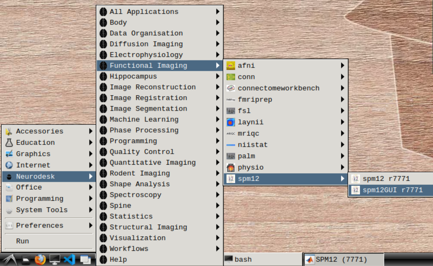
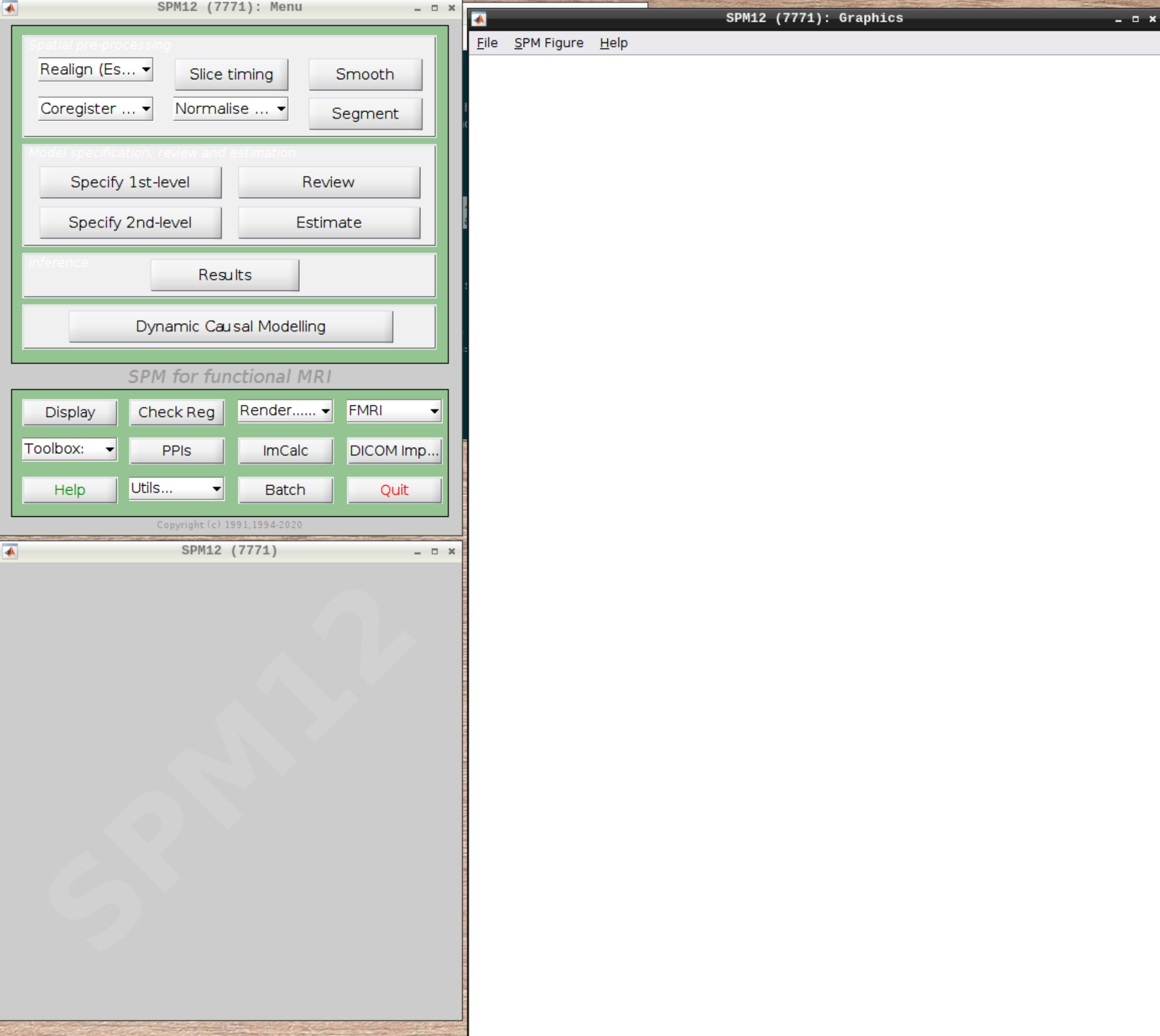
- Open the PhysIO GUI (Neurodesk -> Functional Imaging -> physio -> physioGUI r7771, see screenshot:

- SPM should automatically open up (might take a while). Select ‘fMRI’ from the modality selection screen.
- Press the “Batch Editor” button (see screenshot with open Batch Editor, red highlights)

- NB: If you later want to create a new PhysIO batch with all parameters, from scratch or explore the options, select from the Batch Editor Menu top row, SPM -> Tools -> TAPAS PhysIO Toolbox (see screenshot, read highlights)
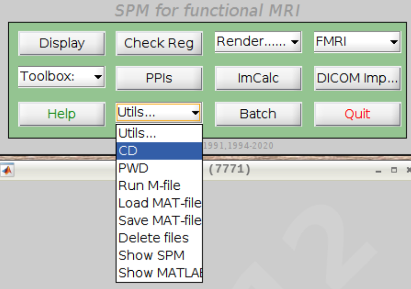
- For now, load an existing example (or previously created SPM Batch File) as follows: It is most convenient to change the working directory of SPM to the location of the physiological logfiles
- In the Batch Editor GUI, lowest row, choose ‘CD’ from the ‘Utils..’ dropdown menu
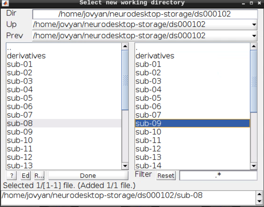
- Navigate to any of the example folders, e.g.,
/opt/spm12/examples/Philips/ECG3T/ and select it - NB: you can skip this part, if you later manually update all input files in the Batch Editor window (resp/cardiac/scan timing and realignment parameter file further down)
- Any other example should also work the same way, just CD to its folder before the next step
- Select File -> Load Batch from the top row menu of the Batch Editor window
- make sure you select the matlab batch file
*_spm_job.<m|mat>, (e.g., philips_ecg3t_spm_job.m and philips_ecg3t_spm_job.mat are identical, either is fine), but not the script.
- Press The green “Play” button in the top icon menu row of the Batch Editor Window
- Several output figures should appear, with the last being a grayscale plot of the nuisance regressor design matrix

- Congratulations, your first successful physiological noise model has been created! If you don’t see the mentioned figure, chances are certain input files were not found (e.g., wrong file location specified). You can always check the text output in the “bash” window associated with the SPM window for any error messages.
Further Info on PhysIO
Please check out the README and FAQ
2.2.5 - A batch scripting example for PhysIO toolbox
Follow this tutorial as an example of how to batch script for the PhysIO toolbox using Neurodesk.
This tutorial was created by Kelly G. Garner.
Github: @kel-github
Twitter: @garner_theory
Getting Setup with Neurodesk
For more information on getting set up with a Neurodesk environment, see hereThis tutorial walks through 1 way to batch script the use of the PhysIO toolbox with Neurodesk.
The goal is to use the toolbox to generate physiological regressors to use when modelling fMRI data.
The output format of the regressor files are directly compatible for use with SPM, and can be adapted to fit the specifications of other toolboxes.
Getting started
This tutorial assumes the following:
- Your data are (largely) in BIDS format
- That you have converted your .zip files containing physiological data to .log files. For example, if you’re using a CMRR multi-band sequence, then you can use this function
- That your .log files are in the subject derivatives/…/sub-…/ses-…/‘func’ folders of aforementioned BIDs structured data
- That you have a file that contains the motion regressors you plan to use in your GLM. I’ll talk below a bit about what I did with the output given by fmriprep (e.g. …_desc-confounds_timeseries.tsv’)
- That you can use SPM12 and the PhysIO GUI to initialise your batch code
NB. You can see the code generated from this tutorial here
1. Generate an example script for batching
First you will create an example batch script that is specific to one of your participants. To achieve this I downloaded locally the relevant ‘.log’ files for one participant, as well as the ‘…desc-confounds_timeseries.tsv’ output for fmriprep for each run. PhysIO is nice in that it will append the regressors from your physiological data to your movement parameters, so that you have a single file of regressors to add to your design matrix in SPM etc (other toolboxes are available).
To work with PhysIO toolbox, your motion parameters need to be in the .txt format as required by SPM.
I made some simple functions in python that would extract my desired movement regressors and save them to the space separated .txt file as is required by SPM. They can be found here.
Once I had my .log files and .txt motion regressors file, I followed the instructions here to get going with the Batch editor, and used this paper to aid my understanding of how to complete the fields requested by the Batch editor.
I wound up with a Batch script for the PhysIO toolbox that looked a little bit like this:

2. Generalise the script for use with any participant
Now that you have an example script that contains the specific details for a single participant, you are ready to generalise this code so that you can run it for any participant you choose. I decided to do this by doing the following:
- First I generate an ‘info’ structure for each participant. This is a structure saved as a matfile for each participant under ‘derivatives’, in the relevant sub-z/ses-y/func/ folder. This structure contains the subject specific details that PhysIO needs to know to run. Thus I wrote a matlab function that saves a structure called info with the following fields:
% -- outputs: a matfile containing a structure called info with the
% following fields:
%    -- sub_num = subject number: [string] of form '01' '11' or '111'
%    -- sess = session number: [integer] e.g. 2
%    -- nrun = [integer] number of runs for that participant
%    -- nscans = number of scans (volumes) in the design matrix for each
%    run [1, nrun]
%    -- cardiac_files = a cell of the cardiac files for that participant
%    (1,n = nrun) - attained by using extractCMRRPhysio()
%    -- respiration_files = same as above but for the resp files - attained by using extractCMRRPhysio()
%    -- scan_timing = info file from Siemens - attained by using extractCMRRPhysio()
%    -- movement = a cell of the movement regressor files for that
%    participant (.txt, formatted for SPM)
To see the functions that produce this information, you can go to this repo here
- Next I amended the batch script to load a given participant’s info file and to retrieve this information for the required fields in the batch. The batch script winds up looking like this:
%% written by K. Garner, 2022
% uses batch info:
%-----------------------------------------------------------------------
% Job saved on 17-Aug-2021 10:35:05 by cfg_util (rev $Rev: 7345 $)
% spm SPM - SPM12 (7771)
% cfg_basicio BasicIO - Unknown
%-----------------------------------------------------------------------
% load participant info, and print into the appropriate batch fields below
% before running spm jobman
% assumes data is in BIDS format

%% load participant info
sub = '01';
dat_path = '/file/path/to/top-level/of-your-derivatives-fmriprep/folder';
task = 'attlearn';
load(fullfile(dat_path, sprintf('sub-%s', sub), 'ses-02', 'func', ...
              sprintf('sub-%s_ses-02_task-%s_desc-physioinfo', sub, task)))

% set variables
nrun = info.nrun;
nscans = info.nscans;
cardiac_files = info.cardiac_files;
respiration_files = info.respiration_files;
scan_timing = info.scan_timing;
movement = info.movement;

%% initialise spm
spm_jobman('initcfg'); % check this for later
spm('defaults', 'FMRI');

%% run through runs, print info and run

for irun = 1:nrun

    clear matlabbatch

    matlabbatch{1}.spm.tools.physio.save_dir = cellstr(fullfile(dat_path, sprintf('sub-%s', sub), 'ses-02', 'func')); % 1
    matlabbatch{1}.spm.tools.physio.log_files.vendor = 'Siemens_Tics';
    matlabbatch{1}.spm.tools.physio.log_files.cardiac = cardiac_files(irun); % 2
    matlabbatch{1}.spm.tools.physio.log_files.respiration = respiration_files(irun); % 3
    matlabbatch{1}.spm.tools.physio.log_files.scan_timing = scan_timing(irun); % 4
    matlabbatch{1}.spm.tools.physio.log_files.sampling_interval = [];
    matlabbatch{1}.spm.tools.physio.log_files.relative_start_acquisition = 0;
    matlabbatch{1}.spm.tools.physio.log_files.align_scan = 'last';
    matlabbatch{1}.spm.tools.physio.scan_timing.sqpar.Nslices = 81;
    matlabbatch{1}.spm.tools.physio.scan_timing.sqpar.NslicesPerBeat = [];
    matlabbatch{1}.spm.tools.physio.scan_timing.sqpar.TR = 1.51;
    matlabbatch{1}.spm.tools.physio.scan_timing.sqpar.Ndummies = 0;
    matlabbatch{1}.spm.tools.physio.scan_timing.sqpar.Nscans = nscans(irun); % 5
    matlabbatch{1}.spm.tools.physio.scan_timing.sqpar.onset_slice = 1;
    matlabbatch{1}.spm.tools.physio.scan_timing.sqpar.time_slice_to_slice = [];
    matlabbatch{1}.spm.tools.physio.scan_timing.sqpar.Nprep = [];
    matlabbatch{1}.spm.tools.physio.scan_timing.sync.nominal = struct([]);
    matlabbatch{1}.spm.tools.physio.preproc.cardiac.modality = 'PPU';
    matlabbatch{1}.spm.tools.physio.preproc.cardiac.filter.no = struct([]);
    matlabbatch{1}.spm.tools.physio.preproc.cardiac.initial_cpulse_select.auto_template.min = 0.4;
    matlabbatch{1}.spm.tools.physio.preproc.cardiac.initial_cpulse_select.auto_template.file = 'initial_cpulse_kRpeakfile.mat';
    matlabbatch{1}.spm.tools.physio.preproc.cardiac.initial_cpulse_select.auto_template.max_heart_rate_bpm = 90;
    matlabbatch{1}.spm.tools.physio.preproc.cardiac.posthoc_cpulse_select.off = struct([]);
    matlabbatch{1}.spm.tools.physio.preproc.respiratory.filter.passband = [0.01 2];
    matlabbatch{1}.spm.tools.physio.preproc.respiratory.despike = true;
    matlabbatch{1}.spm.tools.physio.model.output_multiple_regressors = 'mregress.txt';
    matlabbatch{1}.spm.tools.physio.model.output_physio = 'physio';
    matlabbatch{1}.spm.tools.physio.model.orthogonalise = 'none';
    matlabbatch{1}.spm.tools.physio.model.censor_unreliable_recording_intervals = true; %false;
    matlabbatch{1}.spm.tools.physio.model.retroicor.yes.order.c = 3;
    matlabbatch{1}.spm.tools.physio.model.retroicor.yes.order.r = 4;
    matlabbatch{1}.spm.tools.physio.model.retroicor.yes.order.cr = 1;
    matlabbatch{1}.spm.tools.physio.model.rvt.no = struct([]);
    matlabbatch{1}.spm.tools.physio.model.hrv.no = struct([]);
    matlabbatch{1}.spm.tools.physio.model.noise_rois.no = struct([]);
    matlabbatch{1}.spm.tools.physio.model.movement.yes.file_realignment_parameters = {fullfile(dat_path, sprintf('sub-%s', sub), 'ses-02', 'func', sprintf('sub-%s_ses-02_task-%s_run-%d_desc-motion_timeseries.txt', sub, task, irun))}; %8
    matlabbatch{1}.spm.tools.physio.model.movement.yes.order = 6;
    matlabbatch{1}.spm.tools.physio.model.movement.yes.censoring_method = 'FD';
    matlabbatch{1}.spm.tools.physio.model.movement.yes.censoring_threshold = 0.5;
    matlabbatch{1}.spm.tools.physio.model.other.no = struct([]);
    matlabbatch{1}.spm.tools.physio.verbose.level = 2;
    matlabbatch{1}.spm.tools.physio.verbose.fig_output_file = '';
    matlabbatch{1}.spm.tools.physio.verbose.use_tabs = false;

    spm_jobman('run', matlabbatch);

end
3. Ready to run on Neurodesk!
Now we have a batch script, we’re ready to run this on Neurodesk - yay!
First make sure the details at the top of the script are correct. You can see that this script could easily be amended to run multiple subjects.
On Neurodesk, go to the PhysIO toolbox, but select the command line tool rather than the GUI interface (‘physio r7771 instead of physioGUI r7771). This will take you to the container for the PhysIO toolbox

Now to run your PhysIO batch script, type the command:
run_spm12.sh /opt/mcr/v99/ batch /your/batch/script/named_something.m
Et Voila! Physiological regressors are now yours - mua ha ha!
2.2.6 - Statistical Parametric Mapping (SPM)
A tutorial for running a functional MRI analysis in SPM.
This tutorial was created by Steffen Bollmann.
Email: s.bollmannn@uq.edu.au
Github: @stebo85
Twitter: @sbollmann_MRI
Getting Setup with Neurodesk
For more information on getting set up with a Neurodesk environment, see hereThis tutorial is based on the excellent tutorial from Andy’s Brain book: https://andysbrainbook.readthedocs.io/en/latest/SPM/SPM_Overview.html
Our version here is a shortened and adjusted version for using on the Neurodesk platform.
Download data
First, let’s download the data. We will use this open dataset: https://openneuro.org/datasets/ds000102/versions/00001/download
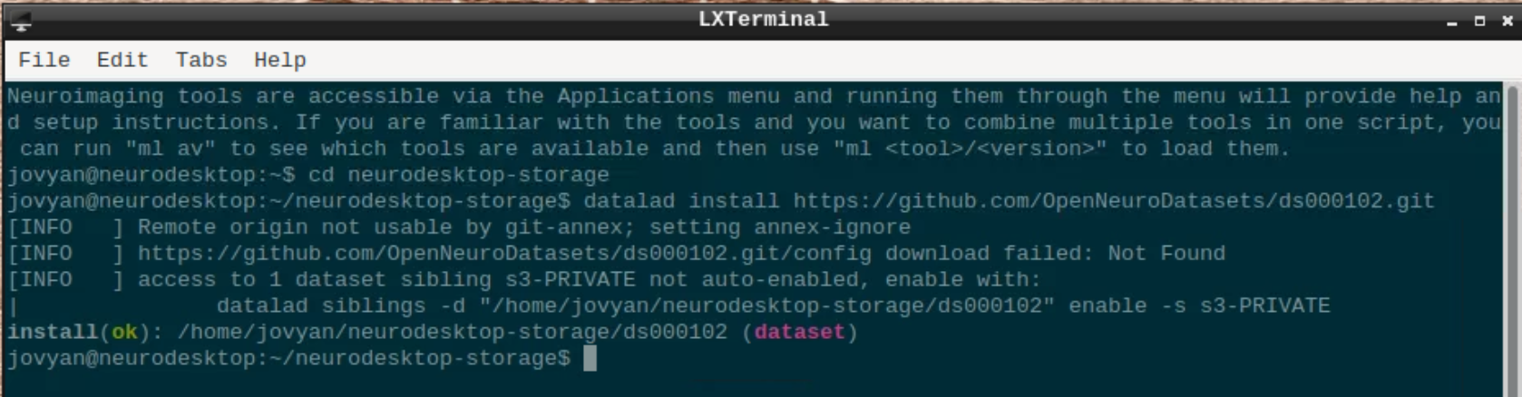
Open a terminal and use datalad to install the dataset:
cd neurodesktop-storage
datalad install https://github.com/OpenNeuroDatasets/ds000102.git
We will use subject 08 as an example here, so we use datalad to download sub-08 and since SPM doesn’t support compressed files, we need to unpack them:
cd ds000102
datalad get sub-08/
gunzip sub-08/anat/sub-08_T1w.nii.gz -f
gunzip sub-08/func/sub-08_task-flanker_run-1_bold.nii.gz -f
gunzip sub-08/func/sub-08_task-flanker_run-2_bold.nii.gz -f
chmod a+rw sub-08/ -R
The task used is described here: https://andysbrainbook.readthedocs.io/en/latest/SPM/SPM_Short_Course/SPM_02_Flanker.html
Starting SPM and visualizing the data
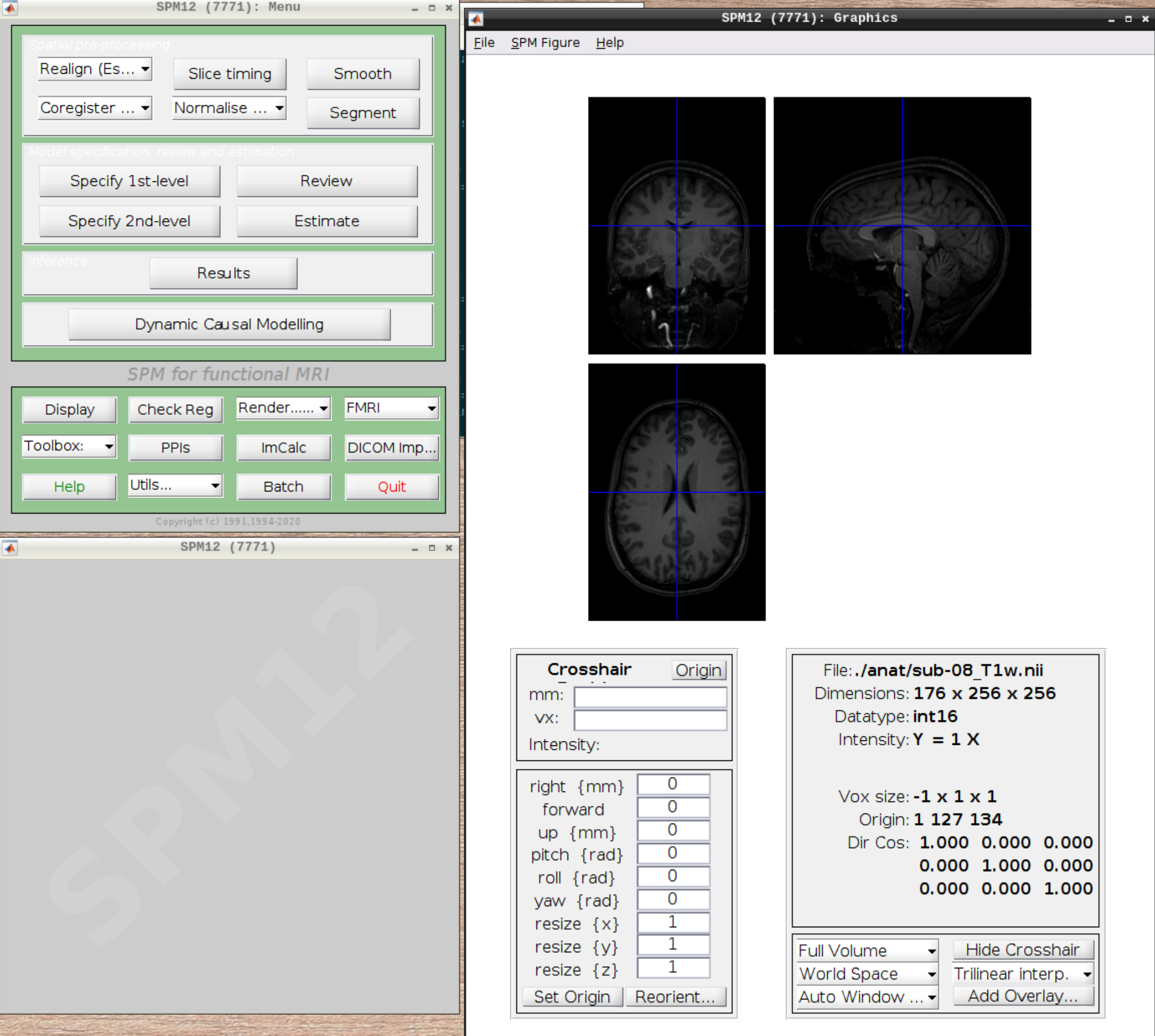
Start spm12GUI from the Application Menu:
When the SPM menu loaded, click on fMRI and the full SPM interface should open up:
For convenience let’s change our default directory to our example subject. Click on Utils and select CD:
Then navigate to sub-08 and select the directory in the right browser window:
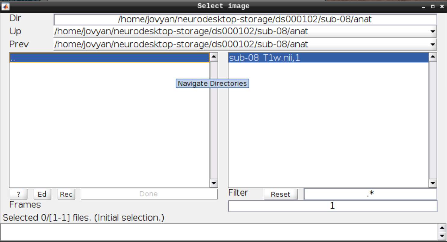
Now let’s visualize the anatomical T1 scan of subject 08 by clicking on Display and navigating and selecting the anatomical scan:
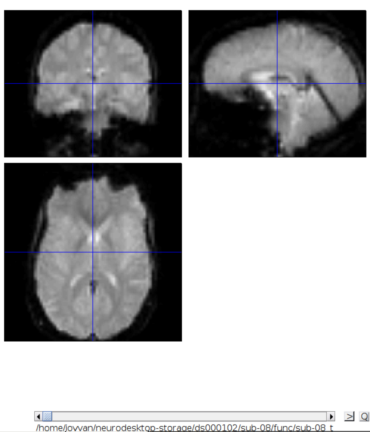
Now let’s look at the functional scans. Use CheckReg and open run-01. Then right click and Browse .... Then set frames to 1:146 and right click Select All
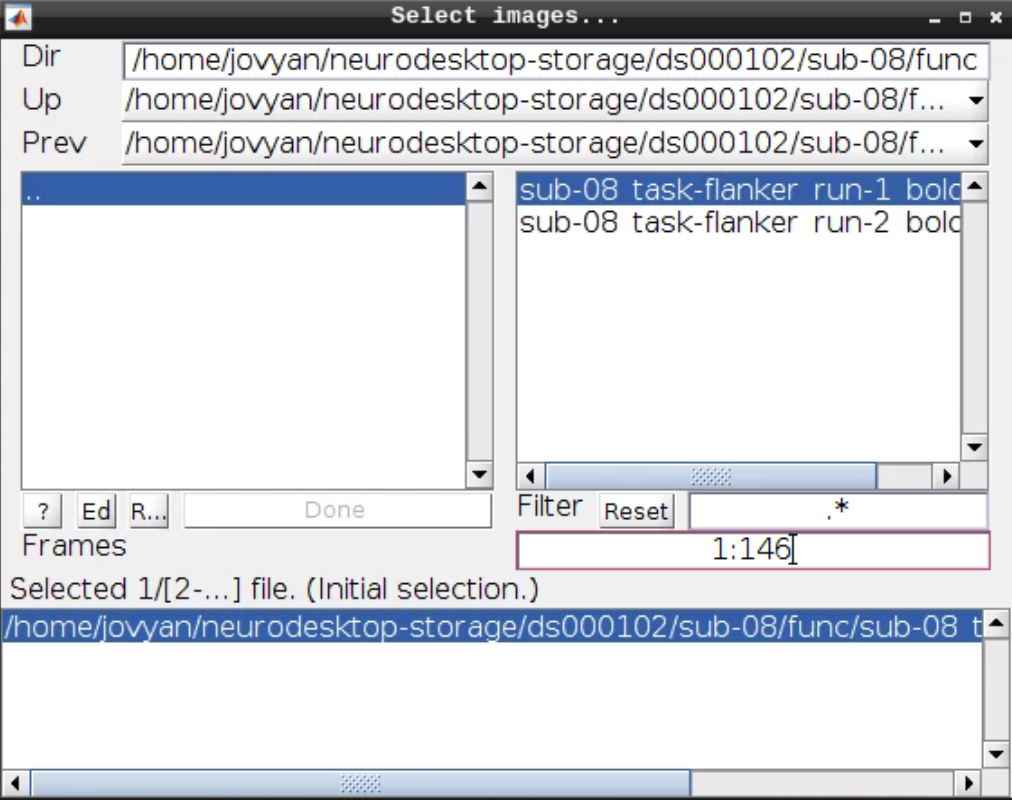
Now we get a slider viewer and we can investigate all functional scans:
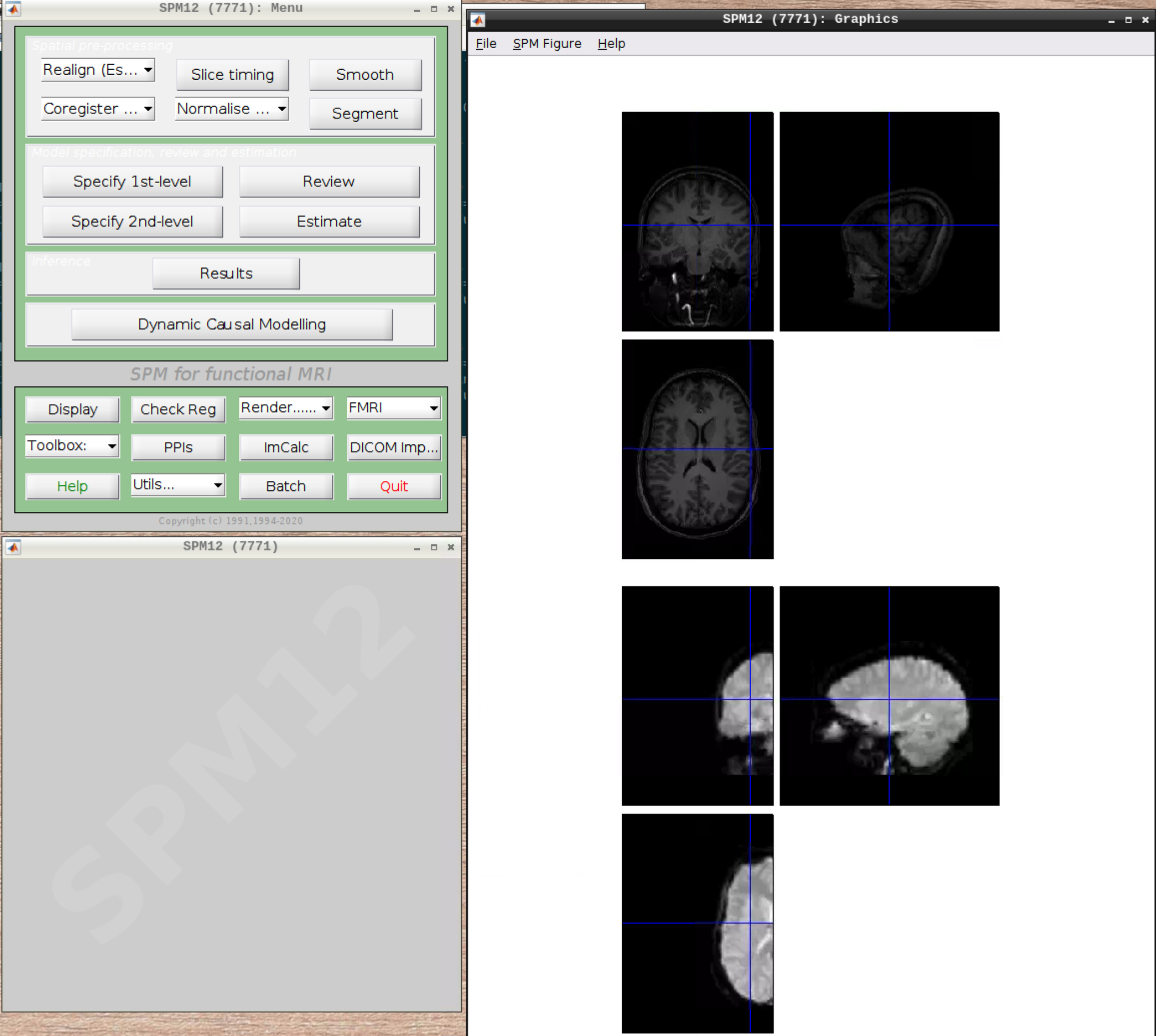
Let’s check the alignment between the anatomical and the functional scans - use CheckReg and open the anatomical and the functional scan. They shouldn’t align yet, because we haven’t done any preprocessing yet:
Preprocessing the data
Realignment
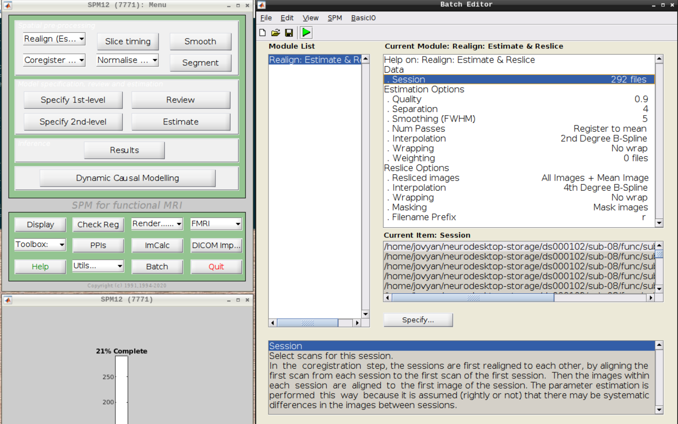
Select Realign (Est & Reslice) from the SPM Menu (the third option):
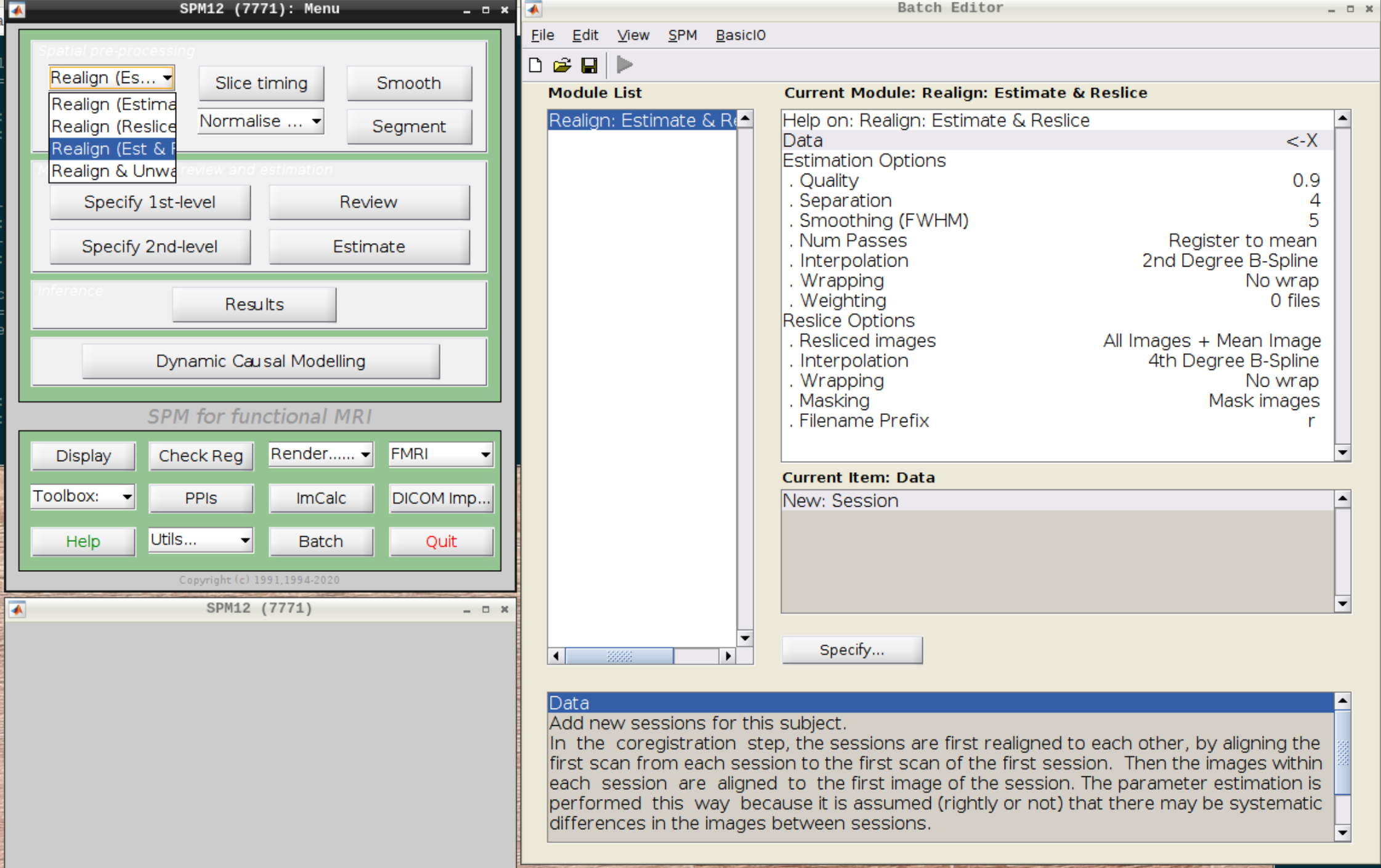
Then select the functional run (important: Select frames from 1:146 again!) and leave everything else as Defaults. Then hit run:
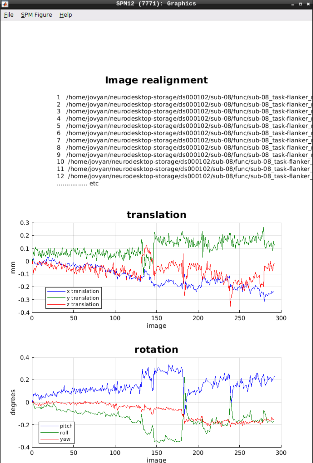
As an output we should see the realignment parameters:
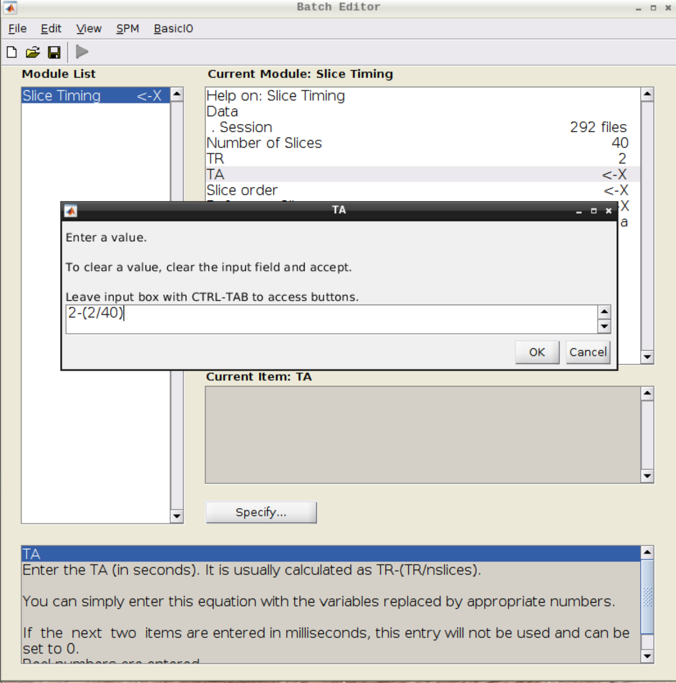
Slice timing correction
Click on Slice timing in the SPM menu to bring up the Slice Timing section in the batch editor:
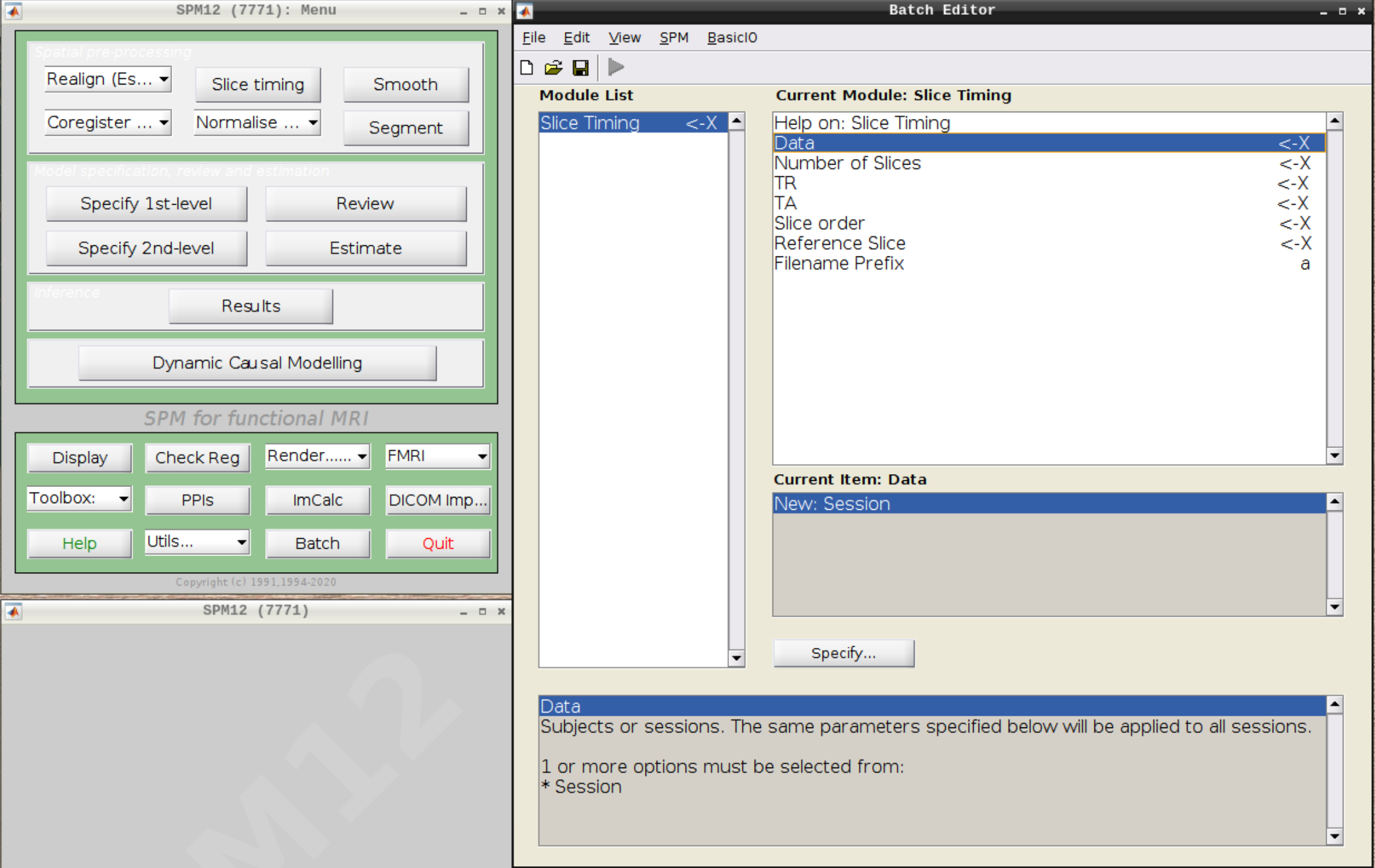
Select the realigned images (use filter rsub and Frames 1:146) and then enter the parameters:
- Number of Slices = 40
- TR = 2
- TA = 1.95
- Slice order = [1:2:40 2:2:40]
- Reference Slice = 1
Coregistration
Now, we coregister the functional scans and the anatomical scan.
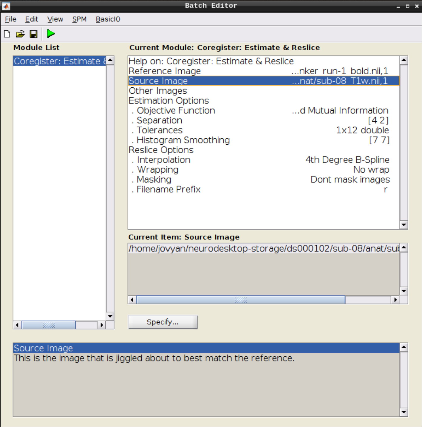
Click on Coregister (Estimate & Reslice) (the third option) in the SPM menu to bring up the batch editor:
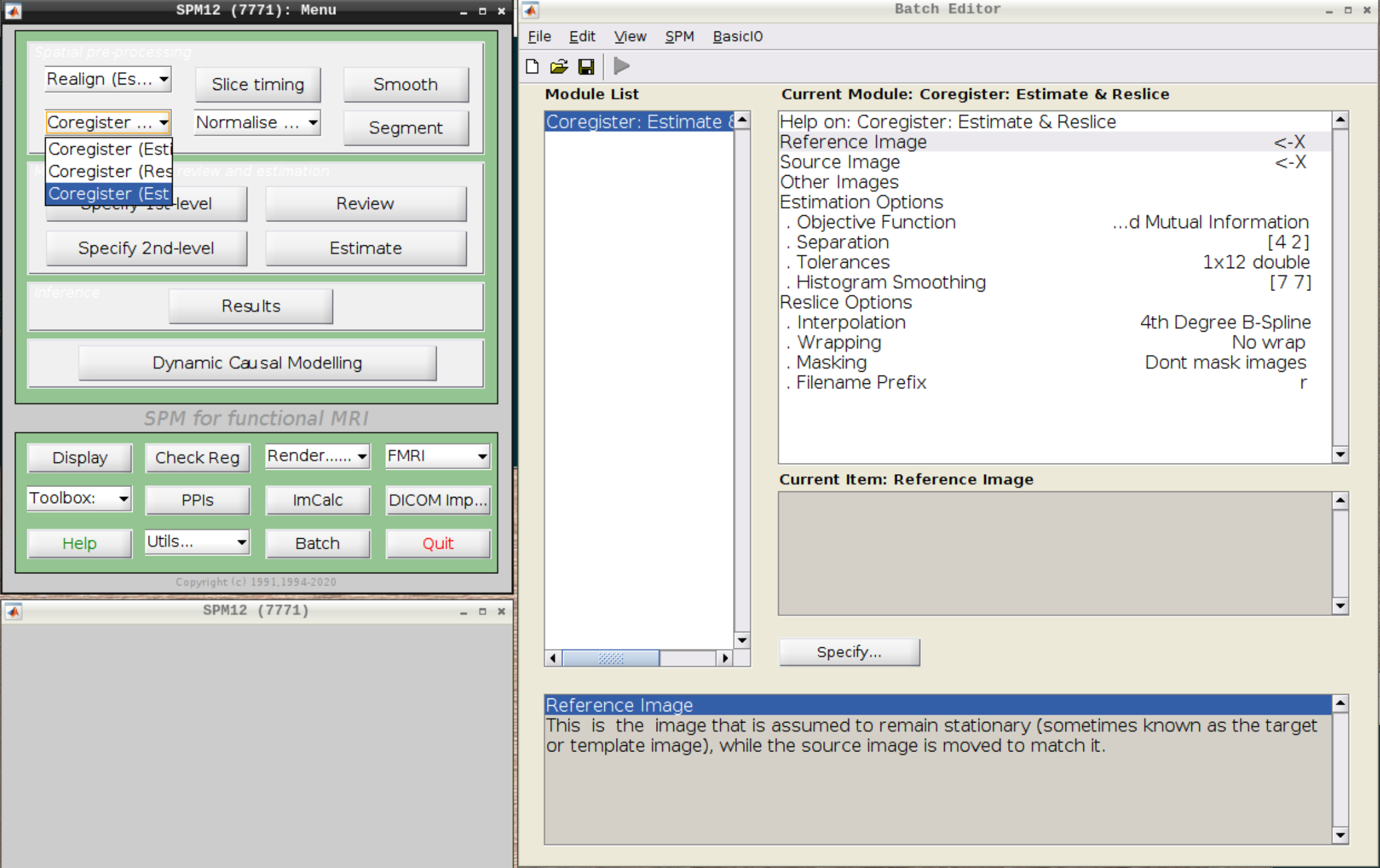
Use the Mean image as the reference and the T1 scan as the source image and hit Play:
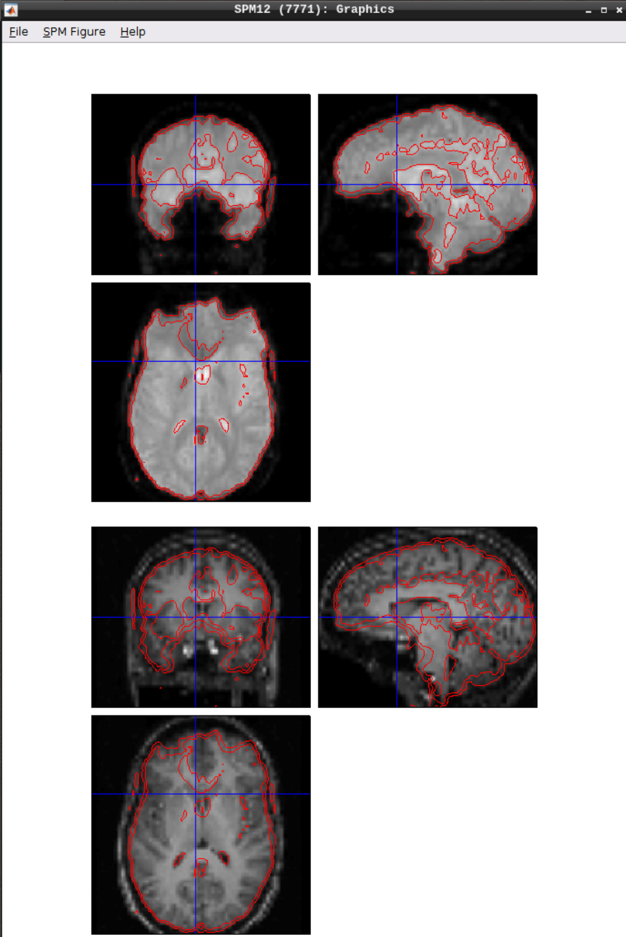
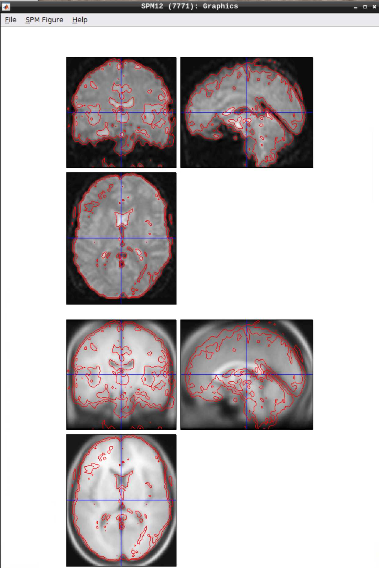
Let’s use CheckReg again and overlay a Contour (Right Click -> Contour -> Display onto -> all) to check the coregistration between the images:
Segmentation
Click the Segmentation button in the SPM menu:
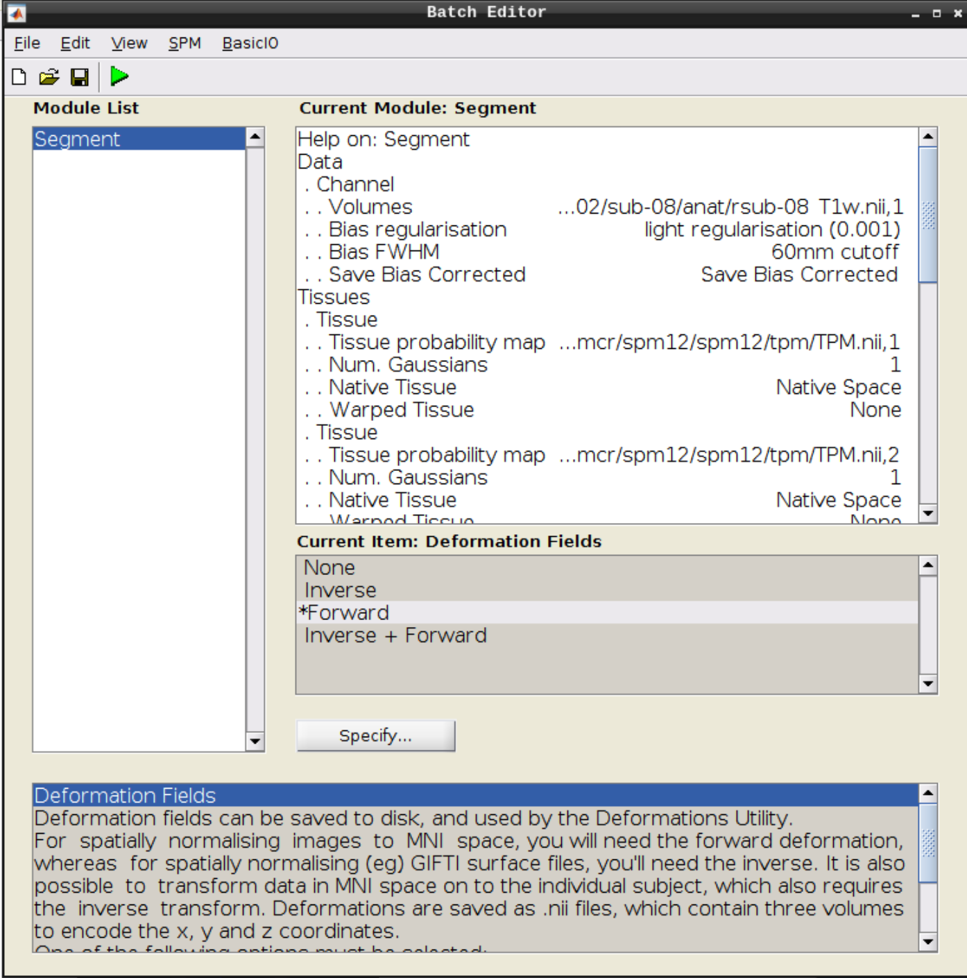
Then change the following settings:
- Volumes = our coregistered anatomical scan rsub-08-T1w.nii
- Save Bias Corrected = Save Bias Correced
- Deformation Fields = Forward
and hit Play again.
Apply normalization
Select Normalize (Write) from the SPM menu:
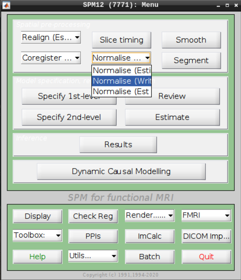
For the Deformation Field select the y_rsub-08 file we created in the last step and for the Images to Write select the arsub-08 functional images (Filter ^ar and Frames 1:146):
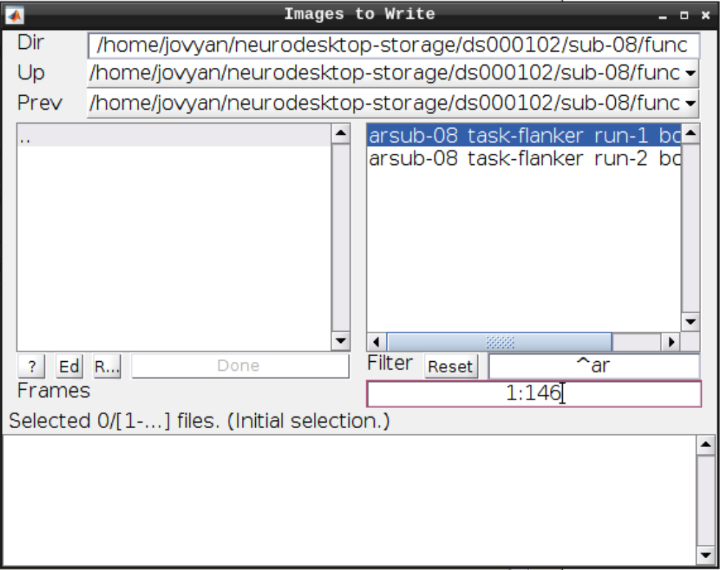
Hit Play again.
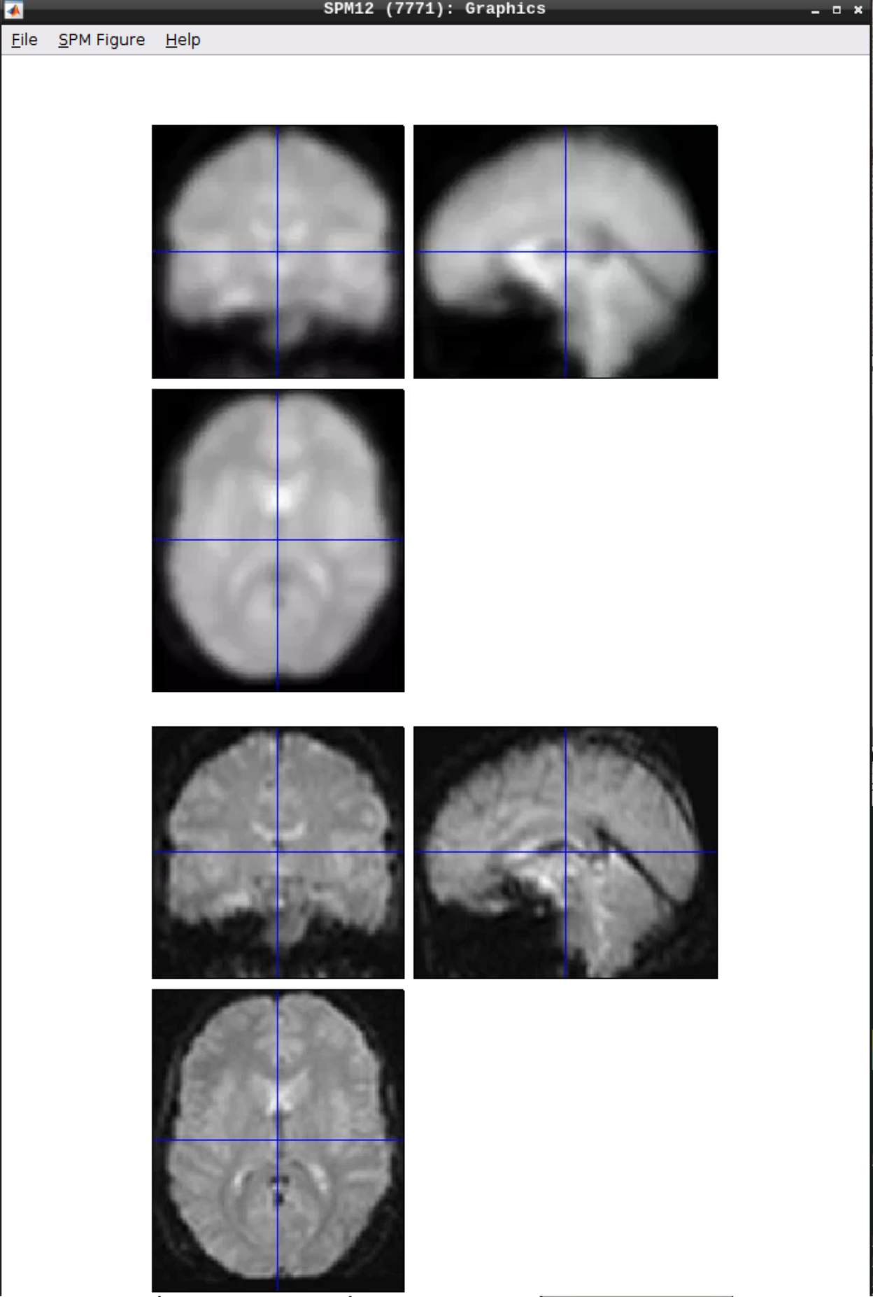
Checking the normalization
Use CheckReg to make sure that the functional scans (starting with w to indicate that they were warped: warsub-08) align with the template (found in /opt/spm12/spm12_mcr/spm12/spm12/canonical/avg305T1.nii):
Smoothing
Click the Smooth button in the SPM menu and select the warped functional scans:
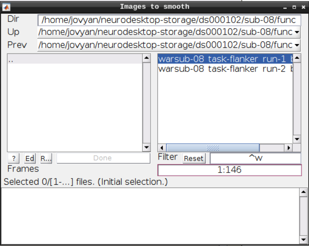
Then click Play.
You can check the smoothing by using CheckReg again:
Analyzing the data
Click on Specify 1st-level - then set the following options:
- Directory: Select the sub-08 top level directory
- Units for design: Seconds
- Interscan interval: 2
- Data & Design: Click twice on New Subject/Session
- Select the smoothed, warped data from run 1 and run 2 for the two sessions respectively
- Create two Conditions per run and set the following:
- For Run 1:
- Name: Inc
- Onsets (you can copy from here and paste with CTRL-V): 0 10 20 52 88 130 144 174 236 248 260 274
- Durations: 2 (SPM will assume that it’s the same for each event)
- Name: Con
- Onsets: 32 42 64 76 102 116 154 164 184 196 208 222
- Durations: 2
- For Run 2:
- Name: Inc
- Onsets: 0 10 52 64 88 150 164 174 184 196 232 260
- Durations: 2
- Name: Con
- Onsets: 20 30 40 76 102 116 130 140 208 220 246 274
- Durations: 2
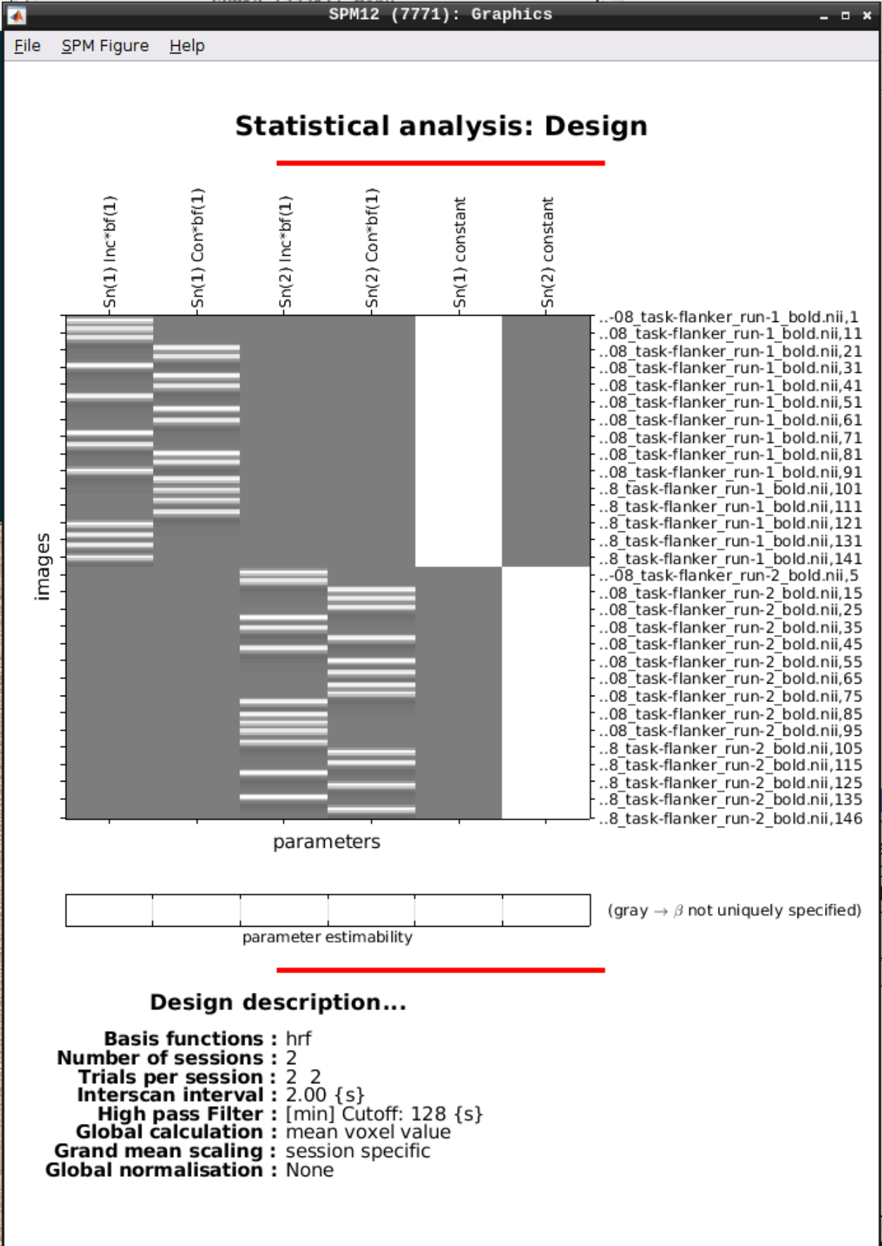
When done, click the green Play button.
We can Review the design by clicking on Review in the SPM menu and selecting the SPM.mat file in the model directory we specified earlier and it should look like this:
Estimating the model
Click on Estimate in the SPM menu and select the SPM.mat file, then hit the green Play button.
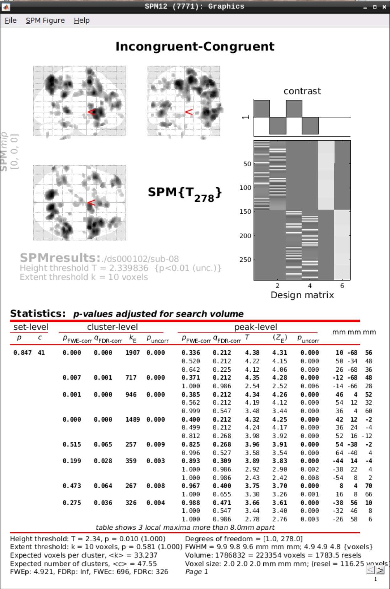
Inference
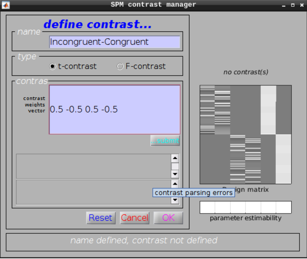
Now open the Results section and select the SPM.mat file again. Then we can test our hypotheses:
Define a new contrast as:
- Name: Incongruent-Congruent
- Contrast weights vector: 0.5 -0.5 0.5 -0.5
Then we can view the results. Set the following options:
- masking: none”
- p value adjustment to control: Click on “none”, and set the uncorrected p-value to 0.01.
- extent threshold {voxels}: 10
2.3 - MRI phase Processing
Tutorials about processing MRI phase
2.3.1 - Quantitative Susceptibility Mapping
Example workflow for Quantitative Susceptibility Mapping
This tutorial was created by Steffen Bollmann and Ashley Stewart.
Github: @stebo85; @astewartau
Web: mri.sbollmann.net
Twitter: @sbollmann_MRI
Getting Setup with Neurodesk
For more information on getting set up with a Neurodesk environment, see hereAn example notebook can be found here:
https://www.neurodesk.org/example-notebooks/structural_imaging/qsmxt_example.html
Please see the above example notebook which provides a detailed QSM tutorial using QSMxT.
2.3.2 - SWI
Example workflow for SWI processing
This tutorial was created by Steffen Bollmann.
Github: @stebo85
Web: mri.sbollmann.net
Twitter: @sbollmann_MRI
Getting Setup with Neurodesk
For more information on getting set up with a Neurodesk environment, see hereDownload demo data
Open a terminal and run:
pip install osfclient
cd /neurodesktop-storage/
osf -p ru43c fetch 01_bids.zip /neurodesktop-storage/swi-demo/01_bids.zip

unzip /neurodesktop-storage/swi-demo/01_bids.zip -d /neurodesktop-storage/swi-demo/
Open the CLEARSWI tool from the application menu:
paste this julia script in a julia file and execute:
cd /neurodesktop-storage/
vi clearswi.jl
hit a or i and then paste this:
using CLEARSWI

TEs = [20]
nifti_folder = "/neurodesktop-storage/swi-demo/01_bids/sub-170705134431std1312211075243167001/ses-1/anat"
magfile = joinpath(nifti_folder, "sub-170705134431std1312211075243167001_ses-1_acq-qsm_run-1_magnitude.nii.gz")
phasefile = joinpath(nifti_folder, "sub-170705134431std1312211075243167001_ses-1_acq-qsmPH00_run-1_phase.nii.gz")

mag = readmag(magfile);
phase = readphase(phasefile);
data = Data(mag, phase, mag.header, TEs);

swi = calculateSWI(data);
# mip = createIntensityProjection(swi, minimum); # minimum intensity projection, other Julia functions can be used instead of minimum
mip = createMIP(swi); # shorthand for createIntensityProjection(swi, minimum)

savenii(swi, "/neurodesktop-storage/swi-demo/swi.nii"; header=mag.header)
savenii(mip, "/neurodesktop-storage/swi-demo/mip.nii"; header=mag.header)
hit SHIFT-Z-Z and run:
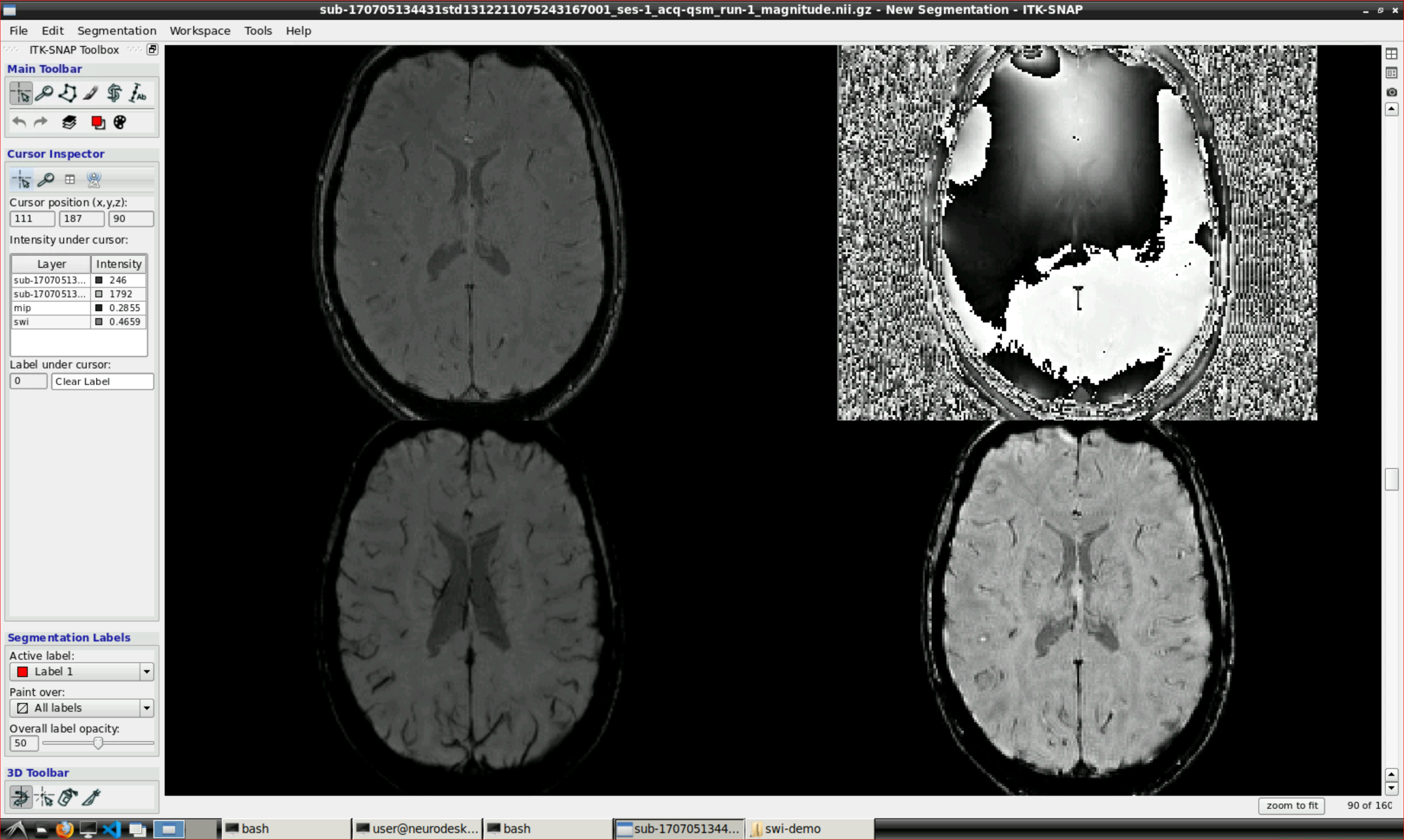
Open ITK snap from the Visualization Application’s menu and inspect the results (the outputs are in swi-demo/swi.nii and mip.nii)
2.3.3 - Unwrapping
MRI Phase Unwrapping
This tutorial was created by Steffen Bollmann.
Github: @stebo85
Web: mri.sbollmann.net
Twitter: @sbollmann_MRI
Getting Setup with Neurodesk
For more information on getting set up with a Neurodesk environment, see hereDownload demo data
Open a terminal and run:
pip install osfclient
cd /neurodesktop-storage/
osf -p ru43c fetch 01_bids.zip /neurodesktop-storage/swi-demo/01_bids.zip

unzip /neurodesktop-storage/swi-demo/01_bids.zip -d /neurodesktop-storage/swi-demo/


mkdir /neurodesktop-storage/romeo-demo/

cp /neurodesktop-storage/swi-demo/01_bids/sub-170705134431std1312211075243167001/ses-1/anat/sub-170705134431std1312211075243167001_ses-1_acq-qsmPH00_run-1_phase.nii.gz /neurodesktop-storage/romeo-demo/phase.nii.gz

cp /neurodesktop-storage/swi-demo/01_bids/sub-170705134431std1312211075243167001/ses-1/anat/sub-170705134431std1312211075243167001_ses-1_acq-qsm_run-1_magnitude.nii.gz /neurodesktop-storage/romeo-demo/mag.nii.gz

gunzip /neurodesktop-storage/romeo-demo/mag.nii.gz
gunzip /neurodesktop-storage/romeo-demo/phase.nii.gz
Using ROMEO for phase unwrapping
Open the ROMEO tool from the application menu and run:
romeo -p /neurodesktop-storage/romeo-demo/phase.nii -m /neurodesktop-storage/romeo-demo/mag.nii -k nomask -o /neurodesktop-storage/romeo-demo/

2.4 - Multimodal Imaging
Tutorials about processing multimodal data (e.g. functional MRI, diffusion, MEG/EEG)
2.4.1 - Using MFCSC
A tutorial for using MFCSC to integrate connectomes from different modalities
This tutorial was created by Oren Civier.
Github: [@civier]
Email: orenciv@gmail.com
More details on MFCSC and this tutorial can be found in the following paper:
Civier O, Sourty M, Calamante F (2023) MFCSC: Novel method to calculate mismatch between functional and structural brain connectomes, and its application for detecting hemispheric functional specialisations. Scientific Reports
https://doi.org/10.1038/s41598-022-17213-z
In short, MFCSC calculates the mismatch between connectomes generated from different imaging modalities. It does it by normalising the connectomes to a common space calculated at group level, and taking into account the role of indirect connectivity in shaping the functional connectomes.
TUTORIAL FOR CONNECTOMES FROM fMRI AND dMRI
Download the “input” folder from the OSF repository (https://osf.io/d7j9n/files/osfstorage)
Launch mfcsc from either “Neurodesk”–>“Diffusion Imaging –> mfsc –> mfcsc 1.1” or “Neurodesk”–>“Functional Imaging –> mfcsc –> mfcsc 1.1” in the start menu.
Run the following command with input being the directory where the input data was downloaded to, and outputdir being the directory where the output should be written to:
mfcsc input/FC_SC_list.txt input/FC input/SC outputdir
- After MFCSC finishes running, the content of outputdir should be identical to the “output” folder in the OSF repository (https://osf.io/d7j9n/files/osfstorage)
It contains connectomes that encode the mismatch between functional and structural connectivity (mFCSC) for every connection.
TUTORIAL FOR CONNECTOMES FROM MEG AND dMRI
Use the MEG connectivity tutorial to generate functional connectomes from your MEG data using MNE tools on Neurodesk (Tutorial in progress: https://github.com/benmslade/neurodesk.github.io/blob/main/content/en/tutorials/electrophysiology/meg_connectivity.md)
Use the structul connectivity tutorial to generate structural connectomes from your dMRI data using MRtrix tools on Neurodesk (https://www.neurodesk.org/tutorials-examples/tutorials/structural_imaging/structuralconnectivity/)
Launch mfcsc from either “Neurodesk”–>“Diffusion Imaging –> mfsc –> mfcsc 1.1” or “Neurodesk”–>“Functional Imaging –> mfcsc –> mfcsc 1.1” in the start menu.
Copy the MEG connectomes into input/MEG and the structural connectomes into input/SC
Create an input/MEG_SC_list.txt file that lists the pairing between MEG and structural connectomes
Run the following command with input being the directory where the input data was downloaded to, and outputdir being the directory where the output should be written to:
mfcsc input/MEG_SC_list.txt input/MEG input/SC outputdir
- After MFCSC finishes running, outputdir will contains connectomes that encode the mismatch between MEG and structural connectivity (mFCSC) for every connection.
CITATIONS
When using MFCSC, authors should cite:
Civier O, Sourty M, Calamante F (2023) MFCSC: Novel method to calculate mismatch between functional and structural brain connectomes, and its application for detecting hemispheric functional specialisations. Scientific Reports
https://doi.org/10.1038/s41598-022-17213-z
Rubinov M, Sporns O (2010) Complex network measures of brain
connectivity: Uses and interpretations. NeuroImage 52:1059-69.
When using the structural connectivity matrices from OSF, authors should cite:
Civier O, Smith RE, Yeh CH, Connelly A, Calamante F (2019) Is removal of weak connections necessary for graph-theoretical analysis of dense weighted structural connectomes from diffusion MRI? NeuroImage http://doi.org/10.1016/j.neuroimage.2019.02.039
… and include the following acknowledgment:
Data were provided by the Human Connectome Project, WU-Minn Consortium (Principal Investigators: David Van Essen and Kamil Ugurbil; 1U54MH091657) funded by the 16 NIH Institutes and Centers that support the NIH Blueprint for Neuroscience Research; and by the McDonnell Center for Systems Neuroscience at Washington University, St. Louis, MO.
When using the functional connectivity matrices from OSF, authors should cite:
Civier O, Sourty M, Calamante F (2023) MFCSC: Novel method to calculate mismatch between functional and structural brain connectomes, and its application for detecting hemispheric functional specialisations. Scientific Reports https://doi.org/10.1038/s41598-022-17213-z
… and include the following acknowledgment:
Data were provided by the Human Connectome Project, WU-Minn Consortium (Principal Investigators: David Van Essen and Kamil Ugurbil; 1U54MH091657) funded by the 16 NIH Institutes and Centers that support the NIH Blueprint for Neuroscience Research; and by the McDonnell Center for Systems Neuroscience at Washington University, St. Louis, MO.
ACKNOWLEDGMENTS
National Health and Medical Research Council of Australia (grant numbers APP1091593 andAPP1117724)
Australian Research Council (grant number DP170101815)
National Imaging Facility (NIF), a National Collaborative Research Infrastructure Strategy (NCRIS) capability at Swinburne Neuroimaging, Swinburne University of Technology.
Victorian Government’s Operational Infrastructure Support
Melbourne Bioinformatics at the University of Melbourne (grant number UOM0048)
Sydney Informatics Hub and the University of Sydney’s high performance computing cluster Artemis
Australian Electrophysiology Data Analytics PlaTform (AEDAPT); Australian Research Data Commons
2.5 - Open Data
Tutorials about publishing and accessing open datasets
2.5.1 - datalad
Using datalad to publish and access open data on OSF
This tutorial was created by Steffen Bollmannn.
Github: @stebo85
Getting Setup with Neurodesk
For more information on getting set up with a Neurodesk environment, see hereDataLad is an open-source tool to publish and access open datasets. In addition to many open data sources (OpenNeuro, CBRAIN, brainlife.io, CONP, DANDI, Courtois Neuromod, Dataverse, Neurobagel), it can also connect to the Open Science Framework (OSF): http://osf.io/
Publish a dataset
First we have to create a DataLad dataset:
datalad create my_dataset

# now add files to your project and then add save the files with datalad
datalad save -m "added new files"
Now we can create a token on OSF (Account Settings -> Personal access tokens -> Create token) and authenticate:
Here is an example how to publish a dataset on the OSF:
# create sibling
datalad create-sibling-osf --title best-study-ever -s osf
git config --global --add datalad.extensions.load next

# push
datalad push --to osf
The last steps creates a DataLad dataset, which is not easily human readable.
If you would like to create a human-readable dataset (but without the option of downloading it as a datalad dataset later on):
# create sibling
datalad create-sibling-osf --title best-study-ever-human-readable --mode exportonly -s osf-export

git-annex export HEAD --to osf-export-storage
Access a dataset
To download a dataset from the OSF (if it was uploaded as a DataLad dataset before):
datalad clone osf://ehnwz

cd ehnwz

# now get the files you want to download:
datalad get .
2.5.2 - osfclient
Using osfclient to publish and access open data on OSF
This tutorial was created by Steffen Bollmannn.
Github: @stebo85
Getting Setup with Neurodesk
For more information on getting set up with a Neurodesk environment, see hereThe osfclient is an open-source tool to publish and access open datasets on the Open Science Framework (OSF): http://osf.io/
Setup an OSF token
You can generate an OSF token under your user settings. Then, set the OSF token as an environment variable:
export OSF_TOKEN=YOURTOKEN
Publish a dataset
Here is an example how to publish a dataset on the OSF:
cd /path/to/dataset
osf init
# enter your OSF credentials and project ID

# now copy your data into the directory, cd into the directory and then run:
osf upload -r ./data osfstorage/data

# beware, hidden files may need to be deleted
Note for those who have used ORCID to create their account / log in
You can still use OSF to upload, but you need to use the TOKEN as the username in osf init (from testing, you don’t need to export the OSF_TOKEN variable).
It won’t ask you for a password.
Note on storage for OSF
The limits are now 5GB for private repo, 50gb for public repo as of 2025.
Access a dataset
To download a dataset from the OSF:
osf -p PROJECTID_HERE_eg_y5cq9 clone .
2.6 - Programming
Tutorials about programming with matlab, julia, and others.
2.6.1 - Conda environments
A tutorial for setting up your conda environments on Neurodesk.
This tutorial was created by Fernanda L. Ribeiro.
Email: fernanda.ribeiro@uq.edu.au
Github: @felenitaribeiro
Twitter: @NandaRibeiro93
Getting Setup with Neurodesk
For more information on getting set up with a Neurodesk environment, see hereThis tutorial documents how to create conda environments on Neurodesk.
Conda/Mamba environment
The default conda environment is not persistent across sessions, so this means any packages you install in the standard environment will disappear after you restart the Jupyterlab instance. However, you can create your own conda environment, which will be stored in your homedirectory, by following the steps on this page. This method can also be used to install additional kernels, such as an R kernel.
- In a Terminal window, type in:

For Python:
mamba create -n myenv ipykernel
#OR
conda create -n myenv ipykernel
or for R:
mamba create -n r_env r-irkernel
#OR
conda create -n r_env r-irkernel
Important: For Python environments, you have to set the ipykernel explicitly or a Python version (like “conda create -n myenv python=3.8”), since a kernel is required. Alternatively, in case it was forgotten, you can add a kernel with:
- To check the list of environments you have created, run the following:
mamba env list
#OR
conda env list
- To activate your conda environment and install the required packages from a provided txt file, run:
For Python:
conda activate myenv
pip install -r requirements.txt
or for R:
conda activate r_env
pip install -r requirements.txt
- Given the available environment, when you open a new Launcher tab, there will be a new Notebook option for launching a Jupyter Notebook with that environment active.

Switching the environment on a Jupyter Notebook is also possible on the top right corner dropdown menu.

2.6.2 - Matlab
A tutorial for setting up your matlab license on Neurodesk.
This tutorial was created by Fernanda L. Ribeiro.
Email: fernanda.ribeiro@uq.edu.au
Github: @felenitaribeiro
Twitter: @NandaRibeiro93
Getting Setup with Neurodesk
For more information on getting set up with a Neurodesk environment, see hereThis tutorial documents how to set up your matlab license on Neurodesk.
Matlab license
Note: You need your own Matlab license to use Matlab in Neurodesk. You can either login to your matlab account or you can provide an institutional network license server if your neurodesk runs within your institution network and ran reach your license server.
a) Institutional network license
run the following command once and replace the address of your license server and the license number
mkdir -p /home/jovyan/Downloads && echo -e "SERVER rtlicense1.university.edu D1234560F6 27007\nUSE_SERVER" > /home/jovyan/Downloads/network.lic
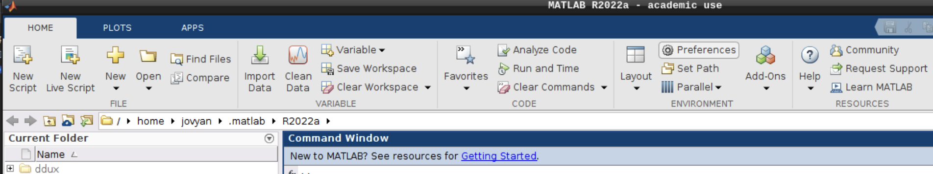
- b) Mathworks account: In the application menu, navigate to Neurodesk → Programming → matlab → matlabGUI 2022a

- Select “Activate automatically using the internet” and hit next.

Then, add your email address and password from your MathWorks account (which you can set up using your university credentials if they provide a license for staff and students).

- Hit next after you select the appropriate license.

- Do not change the login name and hit next.

- Hit confirm, and you are all set!

- To launch the GUI, navigate through the application menu to Neurodesk → Programming → matlab → matlabGUI 2022a
You can use Neurodesk software within Matlab by adding the specific Neurodesk container to your execution Path. For the example of adding the FSL package, this can be done as follows in Matlab:
setenv("PATH",getenv("PATH") + ":/cvmfs/neurodesk.ardc.edu.au/containers/fsl_6.0.7.4_20231005");
Now you can, for example, use fslmaths in Matlab scripts:
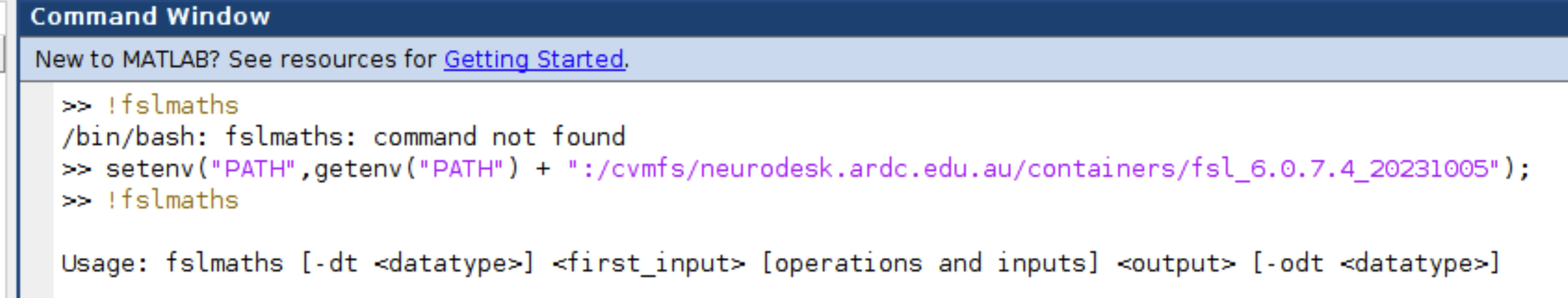
Let us know if this works well for you, and we would be very keen to hear if there is a better way of integrating the lmod system in Matlab.
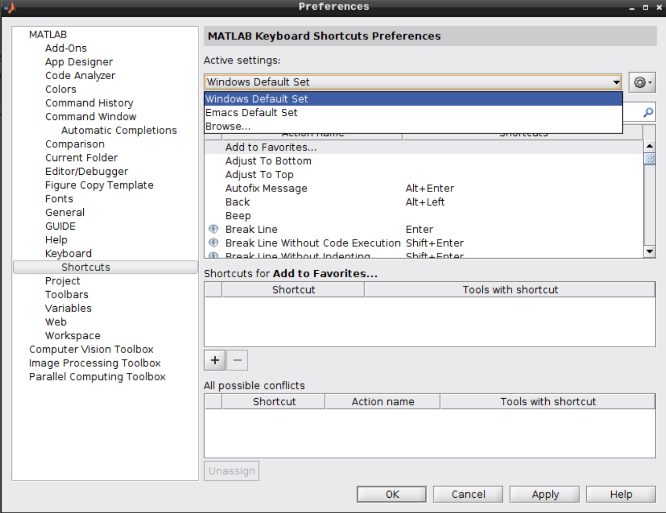
Changing Matlab Keyboard Shortcuts
By default, Matlab uses the emacs keyboard shortcuts in Linux, which might not be what most users expect. To change the keyboard shortcuts to a more common pattern, follow the next steps:
Open the Preferences menu:
Navigate to Keyboard -> Shortcuts and change the active settings from “Emacs Default Set” to “Windows Default Set”:
2.7 - Reproducibility
Tutorials about performing reproducible analyses in general
2.7.1 - Reproducible script execution with DataLad
Using datalad run, you can precisely record results of your analysis scripts.
This tutorial was created by Sin Kim.
Github: @kimsin98
Twitter: @SinKim98
Getting Setup with Neurodesk
For more information on getting set up with a Neurodesk environment, see hereIn addition to being a convenient method of sharing data, DataLad can also help
you create reproducible analyses by recording how certain result files were
produced (i.e. provenance). This helps others (and you!) easily keep track of
analyses and rerun them.
This tutorial will assume you know the basics of navigating the terminal. If
you are not familiar with the terminal at all, check the DataLad Handbook’s
brief guide.
Create a DataLad project
A DataLad dataset can be any collection of files in folders, so it could be
many things including an analysis project. Let’s go to the Neurodesktop storage
and create a dataset for some project. Open a terminal and enter these commands:
$ cd /storage

$ datalad create -c yoda SomeProject
[INFO   ] Creating a new annex repo at /home/user/Desktop/storage/SomeProject
[INFO   ] Running procedure cfg_yoda
[INFO   ] == Command start (output follows) =====
[INFO   ] == Command exit (modification check follows) =====
create(ok): /home/user/Desktop/storage/SomeProject (dataset)
yoda?
-c yoda option configures the dataset according to
the
YODA, a
set of intuitive organizational principles for data analyses that works
especially well with version control.
Go in the dataset and check its contents.
$ cd SomeProject

$ ls
CHANGELOG.md  README.md  code
Create a script
One of DataLad’s strengths is that it assumes very little about your datasets.
Thus, it can work with any other software on the terminal: Python, R, MATLAB,
AFNI, FSL, FreeSurfer, etc. For this tutorial, we will run the simplest Julia
script.
$ ml julia

$ cat > code/hello.jl << EOF
println("hello neurodesktop")
EOF
EOF?
For sake of demonstration, we create the script using
built-in Bash terminal commands only (here document that starts after << EOF
and ends when you enter EOF), but you may use whatever text editor you are
most comfortable with to create the code/hello.jl file.You may want to test (parts of) your script.
$ julia code/hello.jl > hello.txt

$ cat hello.txt
hello neurodesktop
Run and record
Before you run your analyses, you should check the dataset for changes and save
or clean them.
$ datalad status
untracked: /home/user/Desktop/storage/SomeProject/code/hello.jl (file)
untracked: /home/user/Desktop/storage/SomeProject/hello.txt (file)

$ datalad save -m 'hello script' code/
add(ok): code/hello.jl (file)
save(ok): . (dataset)
action summary:
  add (ok: 1)
  save (ok: 1)

$ git clean -i
Would remove the following item:
  hello.txt
*** Commands ***
  1: clean    2: filter by pattern    3: select by numbers    4: ask each   5: quit   6: help
What now> 1
Removing hello.txt
git
git clean is for removing new, untracked files. For
resetting existing, modified files to the last saved version, you would need
git reset --hard.When the dataset is clean, we are ready to datalad run!
$ mkdir outputs

$ datalad run -m 'run hello' -o 'outputs/hello.txt' 'julia code/hello.jl > outputs/hello.txt'
[INFO   ] == Command start (output follows) =====
[INFO   ] == Command exit (modification check follows) =====
add(ok): outputs/hello.txt (file)
save(ok): . (dataset)
Let’s go over each of the arguments:
-m 'run hello': Human-readable message to record in the dataset log.-o 'outputs/hello.txt': Expected output of the script. You can specify
multiple -o arguments and/or use wildcards like 'outputs/*'. This script
has no inputs, but you can similarly specify inputs with -i.'julia ... ': The final argument is the command that DataLad will run.
Before getting to the exciting part, let’s do a quick sanity check.
$ cat outputs/hello.txt
hello neurodesktop
View history and rerun
So what’s so good about the extra hassle of running scripts with datalad run?
To see that, you will need to pretend you are someone else (or you of future!)
and install the dataset somewhere else. Note that -s argument is probably a
URL if you were really someone else.
$ cd ~

$ datalad install -s /neurodesktop-storage/SomeProject
install(ok): /home/user/SomeProject (dataset)

$ cd SomeProject
Because a DataLad dataset is a Git repository, people who download your dataset
can see exactly how outputs/hello.txt was created using Git’s logs.
$ git log outputs/hello.txt
commit 52cff839596ff6e33aadf925d15ab26a607317de (HEAD -> master, origin/master, origin/HEAD)
Author: Neurodesk User <user@neurodesk.github.io>
Date:   Thu Dec 9 08:31:15 2021 +0000

    [DATALAD RUNCMD] run hello

    === Do not change lines below ===
    {
     "chain": [],
     "cmd": "julia code/hello.jl > outputs/hello.txt",
     "dsid": "1e82813d-856f-4118-b54d-c3823e025709",
     "exit": 0,
     "extra_inputs": [],
     "inputs": [],
     "outputs": [
      "outputs/hello.txt"
     ],
     "pwd": "."
    }
    ^^^ Do not change lines above ^^^
Then, using that information, they can re-run the command that created the file
using datalad rerun!
$ datalad rerun 52cf
[INFO   ] run commit 52cff83; (run hello)
run.remove(ok): outputs/hello.txt (file) [Removed file]
[INFO   ] == Command start (output follows) =====
[INFO   ] == Command exit (modification check follows) =====
add(ok): outputs/hello.txt (file)
action summary:
  add (ok: 1)
  run.remove (ok: 1)
  save (notneeded: 1)
git
In Git, each commit (save state) is assigned a long,
unique machine-generated ID. 52cf refers to the commit with ID that starts
with those characters. Usually 4 is the minimum needed to uniquely identify a
commit. Of course, this ID is probably different for you, so change this
argument to match your commit.See Also
- To learn more basics and advanced applications of DataLad, check out the
DataLad Handbook.
- DataLad is built on top of the popular version control tool Git. There
are many great resources on Git online, like this free book.
- DataLad is only available on the terminal. For a detailed introduction on the
Bash terminal, check the BashGuide.
- For even more reproducibility, you can include containers with your dataset
to run analyses in. DataLad has an extension to support script execution in
containers. See here.
2.8 - Spectroscopy
Tutorials about performing MR spectroscopy analyses
2.8.1 - Spectroscopy with lcmodel
Using lcmodel, you can analyze MR spectroscopy data.
This tutorial was created by Steffen Bollmann.
Github: @stebo85
Web: mri.sbollmann.net
Twitter: @sbollmann_MRI
Getting Setup with Neurodesk
For more information on getting set up with a Neurodesk environment, see hereOpen lcmodel from the menu: Applications -> Spectroscopy -> lcmodel -> lcmodel 6.3
run
then run
We packed example data into the container (https://zenodo.org/record/3904443/) and we will use this to show a basic analysis.
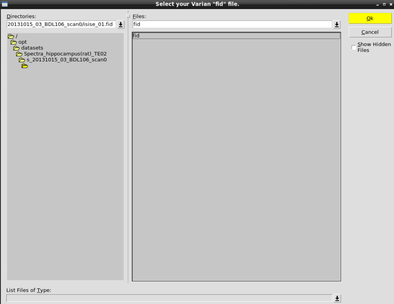
The example data comes in the Varian fid format, so click on Varian:
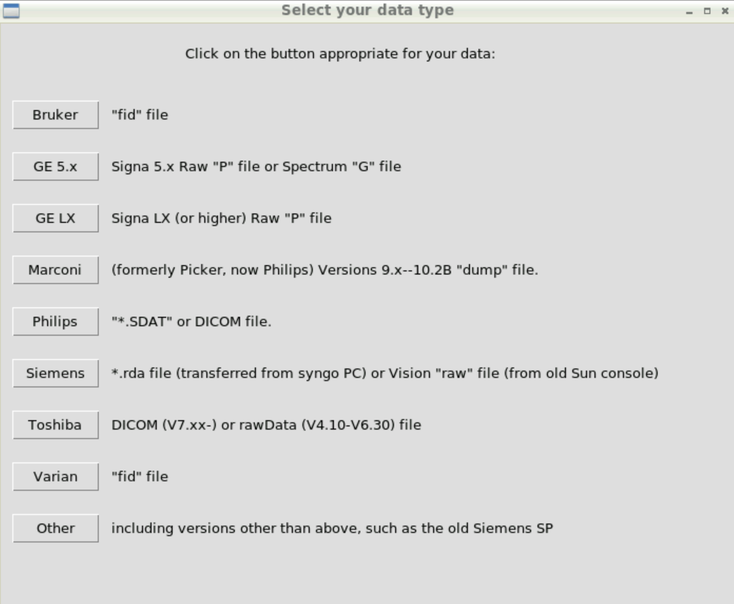
and then select the fid data in: /opt/datasets/Spectra_hippocampus(rat)_TE02/s_20131015_03_BDL106_scan0/isise_01.fid
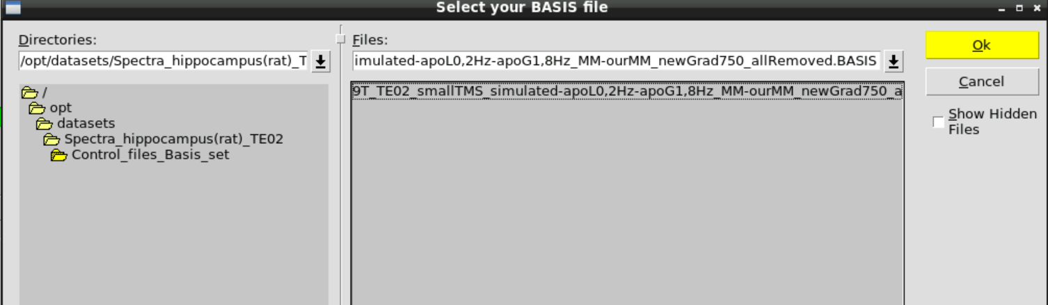
Then Change BASIS and select the appropriate basis set in /opt/datasets/Spectra_hippocampus(rat)_TE02/Control_files_Basis_set
Then hit Run LCModel:
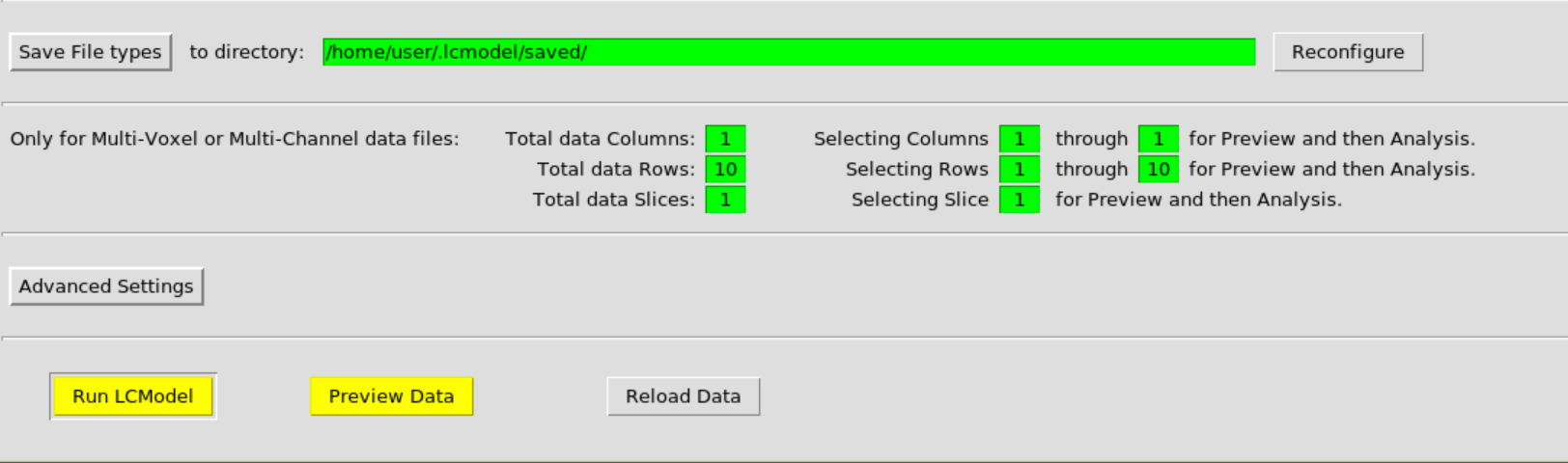
and confirm:
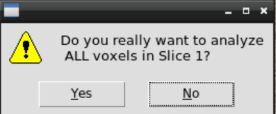
then wait a couple of minutes until the analyzed spectra appear - by closing the window you can go through the results:
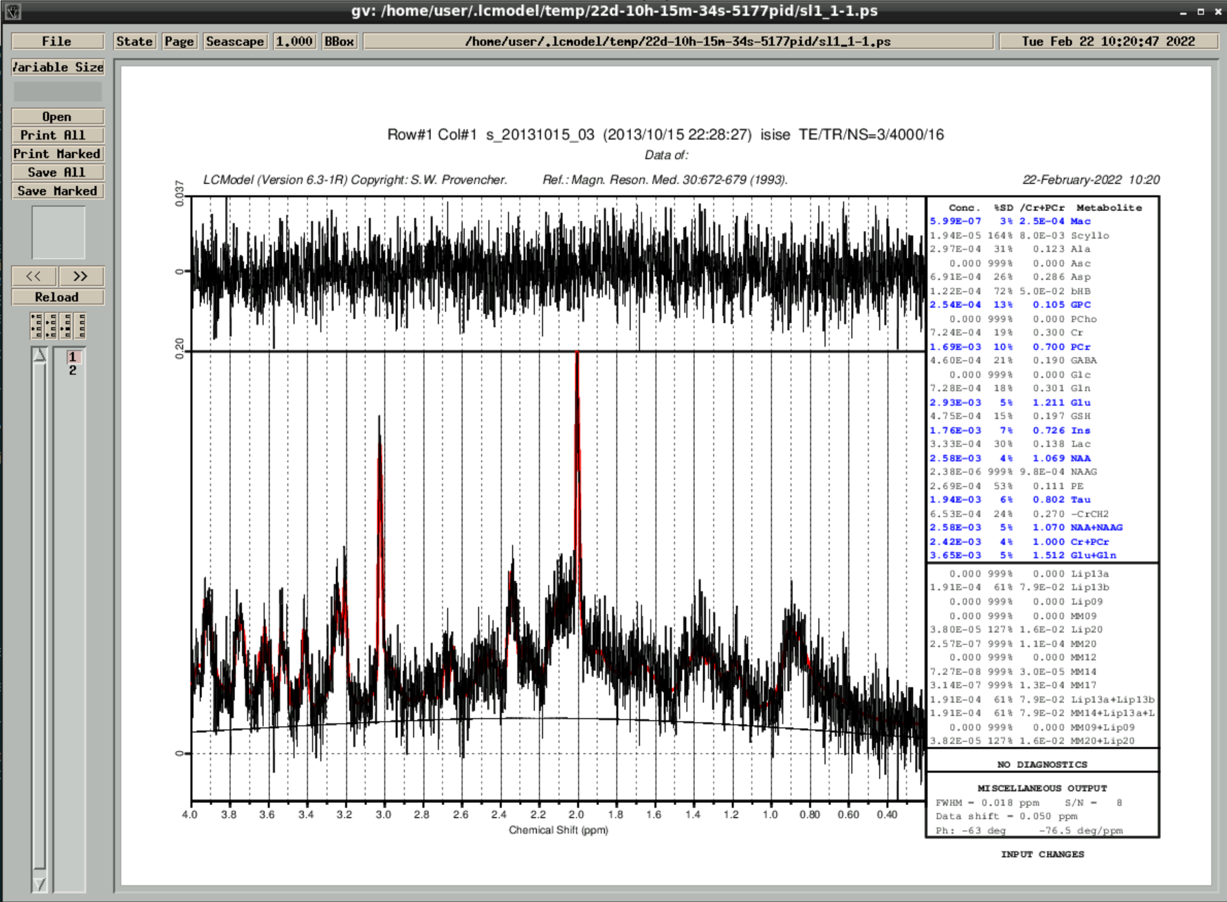
the results are also saved in ~/.lcmodel/saved/
2.8.2 - Spectroscopy pipeline
Using mrsiproc, you can reconstruct and analyze MR spectroscopy data.
This tutorial was created by Korbinian Eckstein.
Github: @korbinian90
Getting Setup with Neurodesk
For more information on getting set up with a Neurodesk environment, see hereProcessing MRSI
bash Part1_ProcessMRSI.sh [ARGUMENTS]
bash Part2_EvaluateMRSI.sh [ARGUMENTS]
Starting Neurodesk
After starting Neurodesk, a JupyterLab instance should open. You can either work from here or open a desktop environment by clicking Neurodesktop under Notebooks. This tutorial uses the desktop.

Running MRSI reconstruction
Open vscode and create and open a new folder under neurodesktop-storage

Info
The processing can either start from reconstructed DICOM files or exported dat files.
A reconstruction of a dat files might look like this:
Part1_ProcessMRSI.sh \
-c /neurodesktop-storage/data/meas_test.dat \
-t /neurodesktop-storage/data/T1/ \
-a /neurodesktop-storage/data/INV1/ \
-b fid_1.300000ms.basis \
-o /neurodesktop-storage/mrsi_proc/ProcessResults/test_files \
-j LCModel_Control_Template.m \
-m "dreid"
The fid_1.300000ms.basis and LCModel_Control_Template.m files are included
Here, we create a new bash file with the default settings and execute it. Copy the contents of this template file to run_mrsi_part1.sh and replace the -c, -t and -a arguments with your own data and set the output path with -o.
#!/bin/bash
# There are two script to process the mrsi data
# First run this script, then run the part 2 script

ml mrsiproc/0.1.0

## The required files are:
# - DAT file / DICOM files
# - T1 (DICOM or .mnc)

## Create own mask (not fully supported yet)
# hd-bet -i /neurodesktop-storage/mrsi_proc/test_files/MP2RAGE/t1.nii.gz -o /neurodesktop-storage/mrsi_proc/test_files/mask.nii.gz -device cpu -mode fast -tta 0
# nii2mnc /neurodesktop-storage/mrsi_proc/test_files/mask.nii.gz /neurodesktop-storage/mrsi_proc/test_files/mask.mnc

Part1_ProcessMRSI.sh \
-c /neurodesktop-storage/data/meas_test.dat \
-t /neurodesktop-storage/data/T1/ \
-a /neurodesktop-storage/data/INV1/ \
-b fid_1.300000ms.basis \
-o /neurodesktop-storage/mrsi_proc/ProcessResults/test_files \
-j LCModel_Control_Template.m \
-m "dreid" \
-L "L2,0.2"

## HINT
# To change the number of threads used by LCModel, change the number in the LCModel_Control_Template.m file (default 8)

## WARNING -s
# The Julia based recontstruction is still experimental! The algorithm is different, and the results are not expected to be identical. It should be identical to the DICOM output from the ICE version.

## WARNING -m
# If a mask file is given, it must be in *.mnc format
# The word "bet" may not be part of the filename of the mask given to the -m flag
# For a 3D mask, it is suggested to use -m "dreid" instead of -m "bet"

## WARNING -t
# The DICOM folder for giving the T1-weighted image must not contain any other files than *.IMA
# The t1-weighted file can be given as *.mnc file as well


## The OPTIONS are
# Usage: %s

# mandatory:
# -c	[csi file]			Format: DAT, DICOM, or .mat. If a .mat file is passed over, it is expected that everything is already performed like coil combination etc.
# 						You can pass over several files of the same type by \'-c \"[csi_path1] [csi_path2] ...\"\'. These files get individually processed and averaged
# 						at the end.
# -b	[basis files]		Format: .BASIS. Used for LCM fitting (for FID)
# -B	[basis files]		Format: .BASIS. Used for LCM fitting (spin echo: for fidesi =  fid + echo)
# -o	[output directory]

# optional:
# -i	[image NORMAL]		Format: DAT or DICOM. The FoV must match that of the CSI file. Used for our coil combination and for creating mask (if no T1 is inputted)
# -f	[image FLIP]		Format: DAT or DICOM. Imaging file FLIP (FOV rotated about -180 deg). Used for correcting gradient delays.
# -v	[VC image]	      	Format: DAT or DICOM. Image of volume or body coil file. Used for sensmap method or for creating mask.
# -t	[T1 images] 		Format: DICOM. Folder of 3d T1-weighted acquisition containing DICOM files. Used for creating mask and for visual purposes. If minc file is given instead of folder, it is treated as the magnitude file.
# -a	[T1 AntiNoise images]	Format: DICOM. Folder of 3d T1-weighted acquisition containing DICOM files. Used for pre-masking the T1w image to get rid of the noise in air-areas.
# -w	[Water Reference]	Format: DAT or DICOM. LCModel 'Do Water Scaling' or separate water quantification (Water maps are created). The same scan as -c [csi file], but without water suppression.
# -m	[mask]			Defines how to create the mask. Options: -m \"bet\", \"thresh\", \"voi\", \"[Path_to_usermade_mask]\". If not set --> no mask used.
# -h 	[100]               	Hamming filter CSI data.
# -r 	[InPlaneCaipPattern_And_VD_Radius]	The InPlaneCaipPattern and the VD_Radius as used in ParallelImagingSimReco.m. Example: \"InPlaneCaipPattern = [0 0 0; 0 0 0; 0 0 1]; VD_Radius = 2;\".
# -R 	[SliceAliasingPattern]
# -g 	[noisedecorr_path]	If this option is used the csi data gets noise decorrelated using noise from passed-over noise file, or if -g \" is given, by noise from the end of the FIDs at the border of the FoV or from the PRESCAN, if available.
# -F    [Nothing]               If this option is set, the spectra are corrected for the first order phase caused by an acquisition delay of the FID-sequences. You must provide a basis set with an appropriate acquisition delay. DONT USE WITH SPIN ECHO SEQUENCES.
# -u	[Nothing]               If a phantom was measured. Different settings used for fitting (e.g. some metabolites are omitted)
# -I	[\"nextpow2\" Or Vector]If nextpow2: Perform zerofilling to the next power of 2 in ROW and COL dimensions (e.g. from 42x42 to 64x64). If vector (e.g. [16 16 1]): Spatially Interpolate to this size.
# -A	[\"\" Or Path]          Perform frequency alignment. If a mnc file is given, use these as B0-map, otherwise shift according to water peak of center voxel.
# -l	[Nothing]               If this option is set, LCModel is not started, everything else is done normally. Useful for only computing the SNR.
# -j	[LCM_ControlFile]       ControlFile telling LCModel how to process the data. for FID
# -J	[LCM_ControlFile]       ControlFile telling LCModel how to process the data. for ECHO
# -X	[XPACE MOTION LOG]       XPACE MOTION LOG
# 							otherwise standard values are assumed. A template file is provided in this package.
# -e	[LineBroadeningInHz]    Apply an exponential filter to the spectra [Hz].
# -s	[threads] [mmap] 		Use the Julia reconstruction version (less RAM usage, different reconstruction algorithm). [threads=auto] can be auto or a number. [mmap=false] can be \"true\", \"false\" or a path.
# -d    [Nothing]				Use the deprecated, old dat file format (before sequence merging, 06/2023)
Then run the script with

This can take several hours for reconstruction and LCModel processing.
Part 2
Continue with the same process for part 2
Template file for part 2
#!/bin/bash

ml mrsiproc/0.1.0

Part2_EvaluateMRSI.sh \
-o neurodesktop-storage/mrsi_proc/ProcessResults/test_files \
-S "Glu,Gln,Raw-abs-csi" \
-N Nifti \
-R \
-b


## The OPTIONS are
# Usage: %s

# mandatory:
# -o	[output directory]

# optional:
# -d	[print_indiv..._flag]   If this option is set, the SNR gets computed by our own program. If the
# 				                print_individual_spectra_flag=1 (by using option -d 1) all spectra for
# 				                computing the SNR are printed.
# -b    [segmentation_matrix_size]
# 				                If segmentation to GM, WM and CSF should be performed.

# -s	[CRLB_treshold_value]	user can set the treshold value for CRLB in the metabolic maps
# -n	[SNR_treshold_value]    If this option is set (user set the value of SNR threshold after the flag),
# 				                SNR binary mask is computed either for LC model SNR or (if the -d flag is set) for
# 				                custom SNR computation method and LCmodel
# -f	[FWHM_treshold_value]   If this option is set (user set the value of FWHM threshold after the flag),
# 				                FWHM binary mask is computed from LCmodel results
# -a    [Control file]          Compute SNR with home-brewed script.
# -l    [local_folder]          Perform some of the file-heavy tasks in \$local_folder/tmpx (x=1,2,3,...) instead of on \$out_dir
#                               directly. This is faster, and if \$out_dir is mounted via nfs4, writing directly to \$out_dir
#                               can lead to timeouts and terrible zombie processes.
# -k	[spectra_stack_range]	If this option is set, the .Coord files from LCmodel are used to create stacks of spectra
# 				                to visualize the fit in corresponding voxels (results stored in form of .eps)
#       				        user can set the starting point of range for stack of spectra for display purposes (in ppm)
# 				                user can set the ending point of range for stack of spectra for display purposes (in ppm)
# 				                Options: \"['fullrange']\", \"[ppm_start; ppm_end]\"
# -r	[non_lin_reg_type]	    If this option is set, the non-linear registration is computed using minctools, Options: -r \"MNI305\", \"MNI152\"
# -w	[compute_reg_only_flag] If this option is set, only the non-linear registration is computed.
# -q	[compute_seg_only_flag] If this option is set, only the segmentation is computed.
# -N    [\"Nifti\" or \"Both\"] Only create nifti-files. If \"Both\" option is used, create minc and nifti. If -N option is not used, creat only mnc files.
# -S    [SpectralMap_flag] 		Create a nifti-file with a map of the LCModel-spectra and -fits to view with freeview as timeseries.\nNeeds freesurfer-linux-centos7_x86_64-dev-20181113-8abd50c, and MATLAB version > R2017b. Can only be used with -N option.
# -u    [UpsampledMaps_flag]	Create upsampled maps by zero-filling (in future more sophisticated methods might be implemented).
# -R    [RatioMaps_flag]		Create Ratio maps.
2.9 - Structural Imaging
Tutorials about processing structural MRI data
2.9.1 - FreeSurfer
Example workflow for FreeSurfer
This tutorial was created by Steffen Bollmann.
Github: @stebo85
Web: mri.sbollmann.net
Twitter: @sbollmann_MRI
Getting Setup with Neurodesk
For more information on getting set up with a Neurodesk environment, see hereFreeSurfer Example using module load (e.g. on an HPC)
Download data:
osf -p bt4ez fetch osfstorage/TOMCAT_DIB/sub-01/ses-01_7T/anat/sub-01_ses-01_7T_T1w_defaced.nii.gz sub-01_ses-01_7T_T1w_defaced.nii.gz
Setup FreeSurfer:
ml freesurfer/7.3.2
export SUBJECTS_DIR=$PWD/freesurfer-output
mkdir $SUBJECTS_DIR
export SINGULARITYENV_SUBJECTS_DIR=$SUBJECTS_DIR
export APPTAINERENV_SUBJECTS_DIR=$SUBJECTS_DIR
Run Recon all pipeline:
recon-all -subject test-subject -i sub-01_ses-01_7T_T1w_defaced.nii.gz -all
When using Freesurfer >8.0.0:
export FS_ALLOW_DEEP=1
export APPTAINERENV_FS_ALLOW_DEEP=$FS_ALLOW_DEEP
export SINGULARITYENV_FS_ALLOW_DEEP=$FS_ALLOW_DEEP
When running on a GPU, make sure to check if this is set:
export neurodesk_singularity_opts='--nv'
Download demo data
Open a terminal and run:
pip install osfclient
osf -p bt4ez fetch TOMCAT_DIB/sub-01/ses-01_7T/anat/sub-01_ses-01_7T_T1w_defaced.nii.gz /neurodesktop-storage/sub-01_ses-01_7T_T1w_defaced.nii.gz
FreeSurfer License file:
Before using Freesurfer you need to request a license here (https://surfer.nmr.mgh.harvard.edu/registration.html) and store it in your homedirectory as ~/.license
FreeSurfer Example
Open FreeSurfer (Neurodesk -> Image Segmentation -> Freesurfer -> Freesurfer 7.1.1)
Setup FreeSurfer license (for example - replace with your license):
echo "Steffen.Bollmann@cai.uq.edu.au
> 21029
>  *Cqyn12sqTCxo
>  FSxgcvGkNR59Y" >> ~/.license

export FS_LICENSE=~/.license
Setup FreeSurfer:
mkdir /neurodesktop-storage/freesurfer-output
source /opt/freesurfer-7.1.1/SetUpFreeSurfer.sh
export SUBJECTS_DIR=/neurodesktop-storage/freesurfer-output
Run Recon all pipeline:
recon-all -subject test-subject -i /neurodesktop-storage/sub-01_ses-01_7T_T1w_defaced.nii.gz -all
2.9.2 - Structural connectivity dMRI
Example workflow for constructing strutural connectivity (Human connectome project: Single subject)
This tutorial was created by Joan Amos.
Email: joan@std.uestc.edu.cn
Github: @Joanone
Getting Setup with Neurodesk
For more information on getting set up with a Neurodesk environment, see hereReferences:
The steps used for this tutorial were from:
Data Description
Reference:
The single subject data (T1w structural and diffusion) used in this tutorial has been minimally preprocessed and was downloaded from the open available source:
db.humanconnectome.org
Download demo data:
Demo data can also be downloaded using these links below.
Assumptions:
- You have neurodesk already running from your chrome browser.
- You have sufficient disk space to successfully implement the structural connectivity.
- The structural and diffusion sample data have been unzipped in the mounted storage directory.
- aparc+aseg.nii.gz
- T1w_acpc_dc_restore_brain.nii.gz
- bvals
- bvecs
- data.nii.gz
N/B: The subfolder used in this tutorial was tagged “Test”
Open a terminal in neurodesk and confirm your input files:
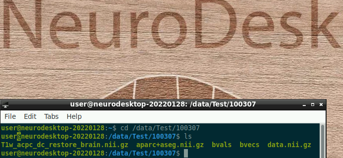
Activate mrtrix3, fsl and afni software versions of your choice in the neurodesk terminal
N/B: mrtrix3 (3.0.3), afni (21.2.00), fsl(6.0.5.1) versions were used in this tutorial. For reproducibility, the same versions can be maintained.
Step 1: Further pre-processing
Extract data.nii.gz to enable memory-mapping. The extracted files are about 4.5GB:
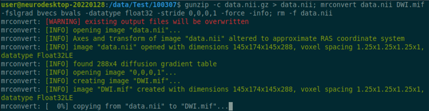
Perform mrconvert:
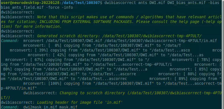
Extract the response function. Uses stride 0,0,0,1:
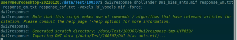
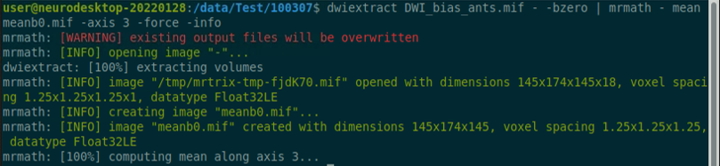
Generate mask:
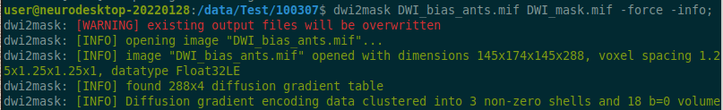
Generate Fibre Orientation Distributions (FODs):
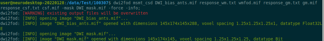
Perform normalization:

Generate a 5 tissue image:
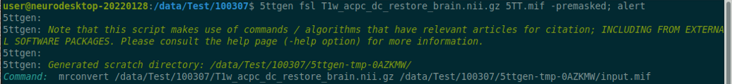
Convert the B0 and 5TT image to a compressed format:
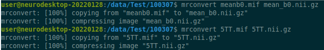
Use “fslroi” to extract the first volume of the segmented dataset which corresponds to the Grey Matter Segmentation:

Use “flirt” command to perform coregisteration:

Convert the transformation matrix to a format readable by MRtrix3:

Coregister the anatomical image to the diffusion image:

Create the seed boundary which separates the grey from the white matter. The command “5tt2gmwmi” denotes (5 tissue type(segmentation) to grey matter/white matter interface):

Step 2: Tractogram construction
The probabilistic tractography which is the default in MRtrix is used in this tutorial. The default method is the iFOD2 algorithm.
The number of streamlines used is 10 million, this was chosen to save computational time:

Proceed to Step 3 when the process above is completed (100%).
Step 3: SIFT2 construction
The generated streamlines can be refined with tcksift2 to counterbalance the overfitting. This creates a text file containing weights for each voxel in the brain:

Step 4: Connectome construction
In constructing the connectome, the desikan-killany atlas which includes the cortical and sub-cortical regions (84 regions) was used.
Copy the “FreeSurferColorLUT.txt” file from the ml freesurfer 7.2.0 singularity container to the subject’s folder:
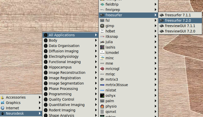

Copy the “fs_default.txt” file from the ml mrtrix3 3.0.3 singularity container to the subject’s folder:

The command labelconvert uses the parcellation and segmentation output of FreeSurfer to create a new parcellated file in .mif format:
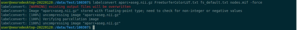
Perform nodes co-registeration:

Create a whole-brain connectome which denotes the streamlines between each parcellation pair in the atlas. The “symmetric” option makes the lower and upper diagonal the same, the “scale_invnodevol” option scales the connectome by the inverse of the size of the node:

Viewing the connectome
The generated nodes.csv file can be viewed outside neurodesk as a matrix in Matlab.
connectome=importdata('nodes.csv');
imagesc(connectome,[0 1])
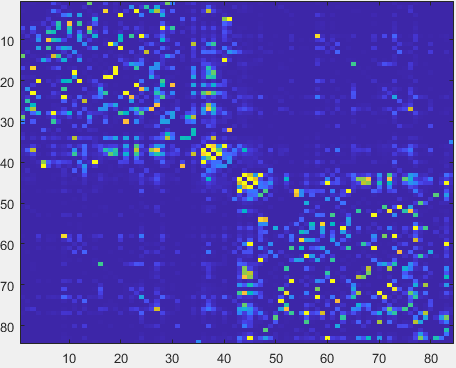
Congratulations on constructing a single subject’s structural connectome with neurodesk! Running multiple subjects would require scripting. Kindly consult the references above.
3 - Contribute Tutorials and Example Notebooks
A brief guide for contributing new tutorials and example notebooks.
Neurodesk welcomes community-contributed content. We aim to collect a wide variety of tutorials and examples representing the spectrum of tools available under the Neurodesk architecture and the diversity in how researchers might apply them. Sharing your expertise helps others learn and supports reproducible research.
- A tutorial: Markdown-based, concise step-by-step documentation integrated into the website, for using specific neuroimaging software on neurodesk with screenshots for visual aid
- An example notebook: Jupyter notebooks that illustrate tool usage or analysis pipelines are stored in a separate repository. These notebooks can be interactive and are ideal for showcasing scripts, visualizations, or code-driven workflows.
How to Contribute
To contribute a new tutorial or example notebook:
Start from the template
Use the tutorial template or the example notebook template as a starting point. They include recommended formatting and structure.
Follow the documentation style
Write clearly and concisely. Include any necessary prerequisites, commands, and expected outputs.
- Tutorials should use Markdown with well-formatted headings, lists, and code blocks
- Notebooks should be well-commented and executable from start to finish
Save your content
Submit your contribution
- Open a pull request to the appropriate repository
- Include a brief summary of what your tutorial or notebook covers
- Check that any links, figures, or code blocks are working and properly rendered
Tips for Good Tutorials
- Focus on a specific tool or workflow
- Include sample commands and outputs
- Keep it as reproducible by using open dataset
- Link to any relevant containers, documentation, or datasets
Attribution
We credit all tutorial contributors on the Contributors page.
If you would like to be listed, please include your name and a short description in your pull request, following this format.
In addition, each example notebook receives a DOI for formal attribution through Zenodo. This ensures that your contribution is citable and can be referenced in academic publications.
Need Help?
If you have questions or would like feedback before submitting, feel free to open a discussion.
Thank you for helping build a more accessible and collaborative neuroimaging community.
3.1 - Contribute Example Notebooks
A brief guide for contributing new example notebooks.
We welcome example notebooks that demonstrate how to use tools within Neurodesk. These notebooks serve as valuable learning resources and promote reproducible workflows across the neuroimaging community.
Example notebooks are hosted in the neurodesk/example-notebooks repository and are intended to be lightweight, self-contained, and easy to follow.
Getting Started
To contribute a new notebook, follow the steps below:
1. Start from the template
Use the official example notebook template as a starting point. It includes guidance on formatting, structure, metadata, and citation instructions.
Each notebook should contain:
- A clear title and short description - aim for a short title that will fit in the left menu
- An overview of the tool or workflow demonstrated
- The container/tool version used
- Code cells with explanatory comments
- Example data (or guidance on how to access it)
Python packages
please consult the python packages included in the base image
see list here. If you are using python packages different than these, be sure to
pip install them in the workflow
2. Follow best practices
- Keep notebooks self-contained and executable top to bottom. Before being published, a Github Action will confirm the Notebook is working.
- Avoid hardcoded file paths where possible
- Use publicly accessible datasets
- Include inline comments and Markdown cells for explanation
For more detail, consult the README in the example-notebooks repository.
Saving and Submitting
Add your completed notebook to the appropriate folder under:
/books/
Open a pull request in the example-notebooks repository
In your pull request, include:
- A short description of your notebook
- Any dependencies or expected output
Attribution
All notebook contributors are acknowledged on the Neurodesk Contributors page.
Please include your name and a short description in your pull request using this format.
Each example notebook receives a DOI for formal citation via Zenodo, ensuring your work is citable in academic contexts.
Need Help?
If you have questions or would like feedback before submitting:
We look forward to your contributions and thank you for supporting open and reproducible neuroimaging.
3.2 - Contribute Tutorials
A brief guide for contributing new tutorials.
We welcome tutorials that walk users through using tools or workflows available in Neurodesk. These tutorials are valuable learning resources that support accessible, reproducible neuroimaging.
Tutorials are written in Markdown and hosted in the neurodesk.github.io:tutorials repository, where they appear as part of the documentation site.
Getting Started
To contribute a new tutorial, follow the steps below:
1. Start from the template
Download the tutorial Markdown template file from GitHub and edit it locally with your own content.
The template includes:
- A frontmatter block with
title, linkTitle, description, and other metadata - A placeholder author attribution block
- Section headings and content structure for a clear tutorial layout
2. Follow best practices
- Use clear, descriptive section headers
- Include step-by-step instructions with commands and screenshots
- Store images in the appropriate
/static/ folder and link them with full paths - Write in plain Markdown, using Hugo formatting where needed
See existing tutorial examples for reference.
Saving and Submitting
Follow the steps for contributing content to Neurodesk.org
Place your completed .md file in the appropriate subfolder under:
/content/en/tutorials-examples/tutorials/
Store any images in a matching subfolder in /static/tutorials-examples/tutorials/
Open a pull request in the neurodesk.github.io repository
In your pull request, include:
- A short summary of your tutorial
- Your name and GitHub handle (if you’d like to be credited)
Attribution
All tutorial contributors are acknowledged on the Contributors page.
To be listed, include your name and a short description in your pull request using this format.
Need Help?
If you have questions or would like feedback before submitting:
We appreciate your contribution to the Neurodesk community and reproducible science.